Country Specific Risk Premium, Taylor Rules, and Exchange Rates

Munich Personal RePEc Archive

Country-Specific Risk Premium, Taylor

Rules, and Exchange Rates

Annicchiarico, Barbara and Piergallini, Alessandro

Department of Economics, University of Rome "Tor Vergata"„

Department of Economics, University of Rome "Tor Vergata",

2010

Online at

https://mpra.ub.uni-muenchen.de/25822/

Country-Specific Risk Premium, Taylor Rules, and

Exchange Rates

∗

Barbara Annicchiarico

University of Rome “Tor Vergata”

Alessandro Piergallini

University of Rome “Tor Vergata”

September 2010

Abstract

The adoption of a Taylor-type monetary policy rule and an inflation target for emerging market economies that choose a flexible exchange rate regime is often advocated. This paper investigates the issue of exchange rate determination when interest-rate feedback rules are implemented in a continuous-time optimizing model of a small open economy facing an imperfect global capital market. It is demon-strated that when a risk premium on external debt affects the monetary policy transmission mechanism, the Taylor principle is not a necessary condition for deter-minacy of equilibrium. On the other hand, it is shown that exchange rate dynamics critically depends on whether monetary policy is active or passive. In terms of optimal monetary policy, it is demonstrated that the degree of responsiveness of the nominal interest rate to inflation should be related to the stock of foreign debt. Specifically, it is optimal to implement a more passive monetary policy stance in response to larger levels of the outstanding foreign-currency-denominated debt.

JEL Classification: F31, F32, E52.

Keywords: Risk Premium on Foreign Debt; Taylor Rules; Exchange Rate Dynamics.

∗_{We wish to thank two anonymous referees, Fabrizio Adriani, Mikael Bask, Andrea Costa, Giuseppe De}

Arcangelis, Ester Faia, Laurence Harris, Giancarlo Marini, Giovanni Piersanti, Giorgio Rodano, Pasquale Scaramozzino, seminar participants at CeFiMS - University of London, DTE - University of Rome “La Sapienza”, and participants at the II RIEF Conference on International Economics and Finance - Univer-sity of Rome “Tor Vergata” for very helpful comments and suggestions. Financial support of the MIUR (Grant No. 2007P8MJ7P 003) is gratefully acknowledged. The usual disclaimer applies.

†_{Corresponding Author: Department of Economics, University of Rome “Tor Vergata”, Via Columbia}

2, 00133 Roma, Italy. E-mail: [email protected]. Phone: +390672595731. Fax:

+39062020500.

‡_{Department of Economics, University of Rome “Tor Vergata”, Via Columbia 2, 00133 Roma, Italy.}

1

Introduction

Modern research on monetary policy provides strong theoretical foundations for the use

of simple interest-rate feedback rules, that specify the setting of the nominal interest

rate as a function of endogenous variables, such as inflation and output. The standard

literature emphasizes the stabilizing role of ‘active’ interest rate rules, that respond to

increases in inflation with a more than one-to-one increase in the nominal interest rate

(e.g., Taylor, 1999; King, 2000; Woodford 2003; McCallum, 2003; Gal´ı, 2008). These

policy rules `a la Taylor (1993) have originally been designed for developed economies. An

important related issue that has attracted growing attention in the recent policy debate

is the design of monetary policy in emerging market and developing economies. The

occurrence of exchange rate crises in emerging economies during the 1990s has warned

against the adoption of ‘soft’ peg exchange rate regimes, as pointed out by Fischer (2001).

In particular, Taylor (2001) argues that ‘for those emerging market economies that do not

choose a policy of a ‘permanently’ fixed exchange rate (perhaps through a currency board

or a common currency (dollarization)), then the only sound monetary policy is one based

on the trinity of a flexible exchange rate, an inflation target, and a monetary policy rule’.

This paper presents an investigation of the dynamic effects of interest-rate feedback

policies of Taylor’s style within a small open economy facing an imperfect world capital

market. Specifically, the analysis is derived in a continuous-time optimizing general

equi-librium framework with flexible exchange rates and an upward-sloping supply curve of

foreign debt. Our model is an extension of the continuous-time closed-economy monetary

framework employed by Benhabib, Schmitt-Groh´e and Uribe (2001) to an open-economy

environment. A discrete-time theoretical setup would not alter the results of our

analy-sis, but would complicate the analysis due the issue concerning the timing convention in

the definition of the stock variables and of real money balances (see, e.g., Carlstrom and

Fuerst, 2001). Our focus on the implications of financial externalities, associated with the

market and developing countries are subject to credit risk, which constrains their

borrow-ing opportunities. The existence of a risk premium on foreign indebtedness in emergborrow-ing

market and developing economies constitutes a fairly well-established stylized fact (e.g.,

Ag´enor and Montiel, 1999; Montiel 2003).

The model considered in this paper is used to examine three relevant issues in

mon-etary theory. First, we investigate dynamic stability to evaluate whether uniqueness of

equilibrium requires that the central bank reacts to inflation with a more than

propor-tional increase in the nominal interest rate (the so-called ‘Taylor principle’), as predicted

by the standard theory on Taylor rules (e.g., Woodford 2003). Second, we reconsider the

issue of exchange rate dynamics in response to exogenous changes in the domestic nominal

interest rate, government spending, the level of productivity, the subjective discount rate,

the foreign nominal interest rate, and the foreign inflation rate. Third, we explore the

properties of the welfare-maximizing interest rate rules and derive the implications for

the optimal policy.

We demonstrate that when a risk premium on external debt affects the monetary

policy transmission mechanism, the Taylor principle is not a necessary condition for

de-terminacy of equilibrium. That is, ‘passive’ interest rate policies, that underreact to

inflation by increasing the nominal interest rate by less than a raise in domestic inflation,

are compatible with saddle-path stability. The economic intuition for this result can be

explained as follows.

Consider first a standard closed-economy framework, with either flexible or sticky

prices. In such a setup, the destabilizing effect of passive monetary policies has the

fol-lowing rationale. If consumers expect a high level of inflation and monetary policy is

passive, the real interest rate declines. As a result of the Euler equation, characterizing

the consumption-saving optimal decision, households reduce savings and increase

con-sumption. The associated increase in aggregate demand causes prices to increase, hence

generate indeterminacy of equilibrium. Monetary policies in the respect of the Taylor

principle are necessary to induce a unique stable equilibrium.

Consider now what occurs in a small-open-economy framework in which the

transmis-sion mechanism of monetary policy is crucially affected by a risk premium on external

debt. When monetary policy is passive, an upward perturbation in inflation causes the

real interest rate to decrease and private consumption to increase, analogously to the

closed-economy case. However, the increase in consumption tends to stimulate foreign

debt accumulation over time, hence leading to an increase in the country-specific risk

premium. This makes the interest rate on foreign debt rise. Ceteris paribus, international

parity conditions precluding arbitrage opportunities require an increase in the domestic

real interest rate, which reduces aggregate demand and inflation. As a result, active

monetary policies are not necessary to guarantee macroeconomic stability.

Despite the fact that saddle-path stability does not require an aggressive interest rate

policy, the study of transitional dynamics we perform demonstrates that exchange rate

adjustment in response to exogenous disturbances depends in a critical way on whether

monetary policy is active or passive. An increase in external debt brings about an increase

in the country-specific risk premium and hence in the nominal interest rate facing the small

open economy. As a consequence, the risk-adjusted interest rate parity condition requires

an increase in the domestic nominal interest rate net of domestic currency depreciation.

The domestic real interest rate must also raise because of the PPP condition. When

monetary policy is active (passive), this raise in the domestic real interest rate may take

place if and only if there is an increase (decrease) in the exchange depreciation rate. This

explains why exchange rate dynamics are crucially affected by whether the monetary

policy stance is active or passive.

We then study the implications for the optimal monetary policy design. We

demon-strate that the degree of responsiveness of the nominal interest rate to inflation should be

imple-ment a more passive monetary policy stance in response to larger levels of the outstanding

foreign-currency-denominated debt. The economic intuition for this result goes as follows.

High external indebtedness causes the country-specific risk premium to rise. As a result,

the interest rate on foreign debt increases. According to the international parity

condi-tions, under an active monetary policy stance the domestic nominal interest rate must

also increase in order ensure a higher real interest rate precluding arbitrage opportunities.

Real money balances decrease, thereby lowering welfare. That is why, in this is case, a

fully accommodating monetary policy is needed.

The scheme of the paper is as follows. Section 2 discusses the paper’s contribution to

the literature. Section 3 presents the model and describes the monetary policy regimes.

Section 4 derives the perfect-foresight macroeconomic equilibrium. Section 5 develops the

steady-state analysis. Section 6 studies the stability properties of the setup and examines

the issue of transitional dynamics. Section 7 studies the optimal monetary policy. Section

8 concludes.

2

Related Literature and Model Choice

In this paper we study exchange rate dynamics in a simple optimizing general equilibrium

monetary model of exchange rate determination, with flexible prices and perfect

compe-tition, extended to include a risk premium on domestic assets and a monetary authority

adopting an interest rate rule. The model used in this paper relates to different strands

of literature.

First, it is related to the literature which explores the conditions under which

interest-rate feedback policy rules may geneinterest-rate macroeconomic instability by causing self-fulfilling

inflation expectations. Notably, Taylor’s (1993) prescription that only active interest rate

rules yield a unique stable equilibrium has been questioned by several works. Benhabib,

is assumed to enter preferences and technology may completely reverse the stabilizing

properties of Taylor-type rules. The present paper contributes to this literature by

inves-tigating whether Taylor’s prescriptions are robust with respect to the presence of external

financial frictions.

Second, the paper is related to the literature focussing on monetary policy design

for small open economies and emerging market economies. Most of these contributions

abstract from the presence of financial externalities, assuming that international asset

markets are complete (e.g., Laxton and Pesenti, 2003; Gal´ı and Monacelli, 2005).

Never-theless, De Paoli (2009) shows that the design of optimal monetary policy is significantly

affected by the asset market structure. Devereux, Lane and Xu (2006) study the welfare

ranking of alternative monetary policy rules for emerging market economies when

finan-cial frictions are operative. The present paper contributes to this literature by analyzing

the issue of dynamic stability in the presence of risk premia on external debt, and by

distinguishing between active and passive interest-rate feedback rules.

Finally, the paper is related to the literature on exchange rate determination. In

particular, it presents a simple and natural microfounded extension of the flexible-price

monetary models of the 1970s (e.g. Frenkel, 1976; Mussa, 1976), along the lines of the

basic-one-good monetary model in small open economy of Turnovsky (1997), where the

purchasing power parity holds continuously and money demand and supply are the key

determinants of exchange rates. By allowing for imperfect substitutability between

do-mestic and foreign assets as a consequence of the existence of a country-specific risk

premium, the paper relates somehow to the early literature on the portfolio balance

mod-els of the 1980s (e.g. Frankel, 1983). By explicitly modelling the optimizing behaviour

of consumers and firms in an intertemporal framework, the model relates to the so-called

new-open-economy-macroeconomics started by Obstfeld and Rogoff (1995). However, in

the traditional literature of exchange rate determination, most results have been derived

sup-ply.1 _{Our model, on the other hand, enables us to examine the implications of financial}

externalities on the exchange rate in small open economies under the assumption that

the monetary authority sets the nominal interest rate as an increasing function of the

inflation rate, consistently with a widely documented empirical evidence. In particular,

we distinguish between active and passive interest rate rules in characterizing exchange

rate dynamics. In this respect, our analysis yields additional insights into the question of

exchange rate dynamics.

3

The Model

Consider a small open economy operating in a world of ongoing inflation and flexible

exchange rates. The economy is described by a one-good-monetary model and consists of

four types of agents: consumers, firms, the government and the central bank. All agents

have perfect foresight.

The domestic economy produces and consumes only one tradeable and non-storable

good. Purchasing power parity (PPP) is assumed to hold at all times:

P =P∗

E, (1)

whereP (P∗

) is the domestic (foreign) price and E is the nominal exchange rate, defined

as units of domestic currency per unit of foreign currency. In percentage terms the PPP

is given by:

π=π∗

+e, (2)

whereπ (π∗

) is the inflation rate of the good in terms of domestic (foreign) currency and

e is the rate of exchange depreciation of domestic currency.

Domestic residents may hold three assets: domestic money, domestic government

1

bonds and foreign assets. Domestic money and government bonds are not held by

foreign-ers. Foreign assets are internationally-traded and are denominated in foreign currency.

However, the home country has not access to a perfect world capital market, but faces an

upward-sloping supply curve of foreign debt, along the lines suggested by Bardhan (1967),

Obstfeld (1982), Bhandari, Haque and Turnovsky (1990), and Turnovsky (1997). From

the standpoint of the borrowing economy, denoting byf the level of real foreign debt and

y domestic output, the nominal interest rate on foreign debtR∗

can then be expressed as

follows:

R∗ =i∗

+σ(f) (3)

wherei∗

is the interest rate prevailing in the world market andσ(f) is the country-specific

risk premium. Function σ(·) is continuous, increasing inf and strictly positive.

International capital mobility implies that a risk-adjusted interest parity of the

fol-lowing type holds:

R=R∗

+e, (4)

where R is the nominal rate of interest on bonds issued by the domestic government.

The infinitely-lived representative consumer faces the following lifetime utility

func-tion: _∞

Z

0

[U(c, ℓ) +V(m)]e−βt

dt, (5)

whereβ is the rate of time preferences andc, ℓandmdenote consumption, labor and real

money balances, respectively. Functions U(·) and V(·) satisfy the following conditions:

Uc >0, Uℓ <0, V′ >0, Ucc<0, Uℓℓ <0, Ucℓ<0, andV′′<0.

The flow budget constraint in real terms is:

•

m+

•

b+a• =wℓ+z−τ −c+ (R−π)b+ (R∗

−π∗

)a−πm, (6)

lump-sum taxes. Notice that, by definition, a = −f. Throughout the paper, for any

generic variable of the model x,x• denotes dx/dt.

The representative agent chooses the optimal plan for c, ℓ, m, b and a in order to

maximize her lifetime utility (5), subject to (6) and given the initial conditions m(0) =

M0

P(0), b(0) =

B0

P(0) and a(0) =

A0

P∗, whereM, B and A denote the nominal stocks of money,

government bonds and foreign assets, respectively. Note that consumers take the rate at

which the country can borrow from abroad as given in making their decisions. In other

words, R∗

is intended to be increasing in the aggregate level of foreign debt, which each

consumer assumes she is unable to influence.

The solution to the consumer’s optimization problem yields the following conditions:

Uc(c, ℓ)−µ= 0, (7)

Uℓ(c, ℓ) +wµ= 0, (8)

V′

(m)−µπ =−µ• +µβ, (9)

µ(R−π) = −µ• +µβ, (10)

µ(R∗

−π∗

) =−µ• +µβ, (11)

together with the flow budget constraint (6), the initial conditions and the transversality

conditions:

lim

t→∞µme −_βt

= lim

t→∞µbe −_βt

= lim

t→∞µae −_βt

= 0, (12)

where µe−βt _{is the discounted Lagrange multiplier associated with the wealth}

accumula-tion equaaccumula-tion (6).

Perfectly competitive firms face a standard neoclassical production function of labor:

where y denotes output, φ′

(·) >0, φ′′

(·)< 0, and Λ is a positive technology parameter.

Each firm hires labor in order to maximize profits. At the optimum, labor marginal

productivity is equal to the real wage rate Λφ′

(ℓ) =w.

The domestic government faces the following flow budget constraint expressed in real

terms:

•

m+

•

b =g−τ + (R−π)b−πm, (14)

where g is government spending. The government is assumed to adopt a tax policy

consisting in balancing the budget at all times:

τ =g+ (R−π)b−πm. (15)

The monetary authorities set the nominal interest rate as an increasing function of

the inflation rate, as in Benhabib, Schmitt-Groh´e and Uribe (2001):

R=i+ρ(π), (16)

where ρ(·) is continuous, non-decreasing, and there exists at least one π >−β such that

i+ ρ(π) = β +π; i is a positive parameter capturing exogenous deviations from the

feedback component of the rule. Following Leeper (1991), the interest rate rule (16) is

‘active (‘passive’) ifρ′

>(<)1. In other words, under an active (passive) monetary policy,

the central bank responds to inflation by raising (lowering) the real interest rate.

The dynamic equation describing the accumulation of net foreign assets is given by

the trade balance plus interest payments:

•

a=y−c−g+ (R∗

−π∗

We can rewrite (17) in terms of net foreign debt accumulation as:

•

f =c+g−y+ (R∗

−π∗

)f. (18)

4

Macroeconomic Equilibrium

Combining the set of optimality conditions (7)-(11) together with the interest rate on

foreign debt function (3), the international parity conditions (2) and (4), the production

function (13), the monetary policy rule (16), and the foreign debt accumulation equation

(18), the perfect-foresight equilibrium can be described as follows:

•

µ=µβ −(i∗

+σ(f)−π∗

)µ, (19)

•

f =c+g−Λφ(ℓ) + (i∗

+σ(f)−π∗

)f, (20)

c=c(µ,Λ), cµ, cΛ <0, (21)

ℓ=ℓ(µ,Λ), ℓµ, ℓΛ >0, (22)

m=m(µ) + ρ

′

ρ′

−1η(i ∗

, f, i, π∗

), mµ<0, ηi∗, η_f <0, η_i, η_π∗ >0, (23)

e= 1

ρ′

−1ǫ(i ∗

, f, i, π∗

), ǫi∗, ǫ_f >0, ǫ_i, ǫ_π∗ <0, (24)

where (19) and (20) are the pair of equations describing the evolution of the economy

over time and (21)-(24) describe the equilibrium paths for consumption, work effort, real

money balances and the rate of exchange depreciation of domestic currency, respectively.

5

Steady-State Analysis

Under the assumption of perfect foresight, the transitional dynamics of the model

de-pends in part on the expectations of the long-run steady state. This Section derives the

steady-state equilibrium and the long-run effects of changes in both domestic and foreign

exogenous variables.

The steady state of the economy is obtained when the shadow value of wealth is

constant and external debt accumulation ceases, that is whenµ• = •

f = 0. From (19)-(24),

the steady state consists of the following set of relationships:

β =i∗

+σ(f)−π∗

, (25)

Λφ(ℓ(µ,Λ)) = (i∗

+σ(f)−π∗

)f+c(µ,Λ) +g, (26)

c=c(µ,Λ), (27)

ℓ =ℓ(µ,Λ), (28)

y= Λφ(ℓ), (29)

m=m(µ) + ρ

′

ρ′₋ 1η

¡

i∗

, f , i, π∗¢

, (30)

e= 1

ρ′

−1ǫ(i ∗

, f , i, π∗

). (31)

Equations (25)-(31) jointly determine the steady-state equilibrium solutions for µ, f, c,

ℓ, y, m and e as functions of the rate of time preference β, the technology parameter Λ,

public spending g, the monetary policy rule exogenous component i, foreign inflation π∗ ,

and the interest rate prevailing in the world marketi∗ .

To study exchange rate dynamics, it is convenient to write down the long-run

re-sponses to changes in exogenous variables of foreign debt and of the rate of depreciation,

df di = 0,

df

dβ =

1

σ′ >0,

df

dΛ =

df

dg = 0, (32)

de

di =−

1

ρ′

−1 <(>)0,

de

dβ =

1

ρ′

−1 >(<)1 if ρ >(<)1 and

de

dΛ =

de

dg = 0. (33)

On the other hand, the responses to changes in the foreign variables are given by:

df dπ∗ =

1

σ′ >0,

df di∗ =−

1

σ′ >0, (34)

de

dπ∗ =−1,

de

di∗ = 0. (35)

The long-run responses of all endogenous variables of the economy to changes in the

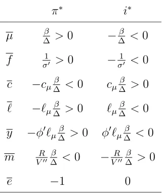
exogenous variables of both domestic and foreign origin are reported in Tables 1 and 2,

respectively, where ∆≡ −σ′

(cµ(µ,Λ)−Λφ

′

ℓµ(µ,Λ))>0. Full derivations are developed

in Appendix B.

6

Transitional Dynamics

Linearizing the differential equations (19)-(20) around the steady-state equilibrium©

µ, fª

yields:    • f • µ   =   

β+σ′

f cµ(µ,Λ)−Λφ

′

ℓµ(µ,Λ)

−σ′

µ 0      

f−f

µ−µ





. (36)

The above system displays one predetermined variable, f, and one jumping variable, µ.

In order to have a unique perfect-foresight equilibrium in the neighborhood of the steady

state (i.e. saddle-path stability), the Jacobian of the system must have eigenvalues of

opposite sign. This property is satisfied by the system (36), since the determinant of the

Jacobian, given by σ′

µ[cµ(µ,Λ)−Λφ

′

ℓµ(µ,Λ)], is negative. The Taylor principle, ρ′ >1,

is not necessary to bring about equilibrium determinacy. Intuitively, this is because the

time path of external debt and the international parity conditions. Whether monetary

policy is active or passive is immaterial for determinacy.

Focusing now on the stable path, the solutions for f and e are given by:

f =f +¡

f0−f

¢

eλt, (37)

e=e+ 1

ρ′

−1ǫf

¡

f −f¢

, (38)

where λ < 0 is the stable eigenvalue and f0 is the initial condition on foreign debt (see

Appendix C for full derivations). Using the steady-state multipliers given by (32)-(35),

the impact effects on the rate of depreciation of changes in domestic and foreign variables

are, respectively:

de(0)+

di =−

1

ρ′

−1 <(>)0 if ρ >(<)1,

de(0)+

dβ =

de(0)+

dΛ =

de(0)+

dg = 0, (39)

de(0)+

dπ∗ =−

ρ′

ρ′₋₁ <(>)0,

de(0)+

di∗ =

1

ρ′₋₁ >(<)0 if ρ >(<)1. (40)

The impact effects on all endogenous variables of changes in domestic and foreign variables

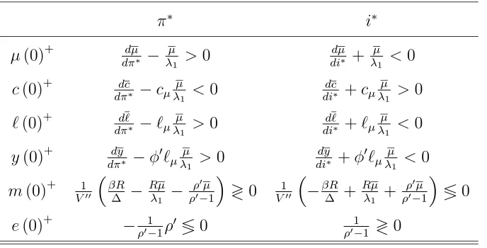
are summarized in Tables 3 and 4 (see Appendix D for details).

From the analysis of both the steady-state equilibrium and the transitional dynamics,

it emerges that the dynamic behavior of the nominal exchange rate critically depends upon

whether the monetary-policy reaction coefficient ρ′

is above or below unity. Examining

(38), in fact, the exchange depreciation rate is correlated with foreign debt, along the

transitional path towards the steady-state equilibrium, with a coefficient, ǫf/(ρ′−1),

which is greater (lower) than zero if ρ′

>(<) 1. An intuitive explanation is the following.

A change in external indebtedness alters the international parity conditions given by

the risk-adjusted interest rate parity, thereby influencing exchange rate dynamics. In

particular, an increase in foreign debt causes the country-specific risk premium to raise,

brings about an increase in the domestic nominal interest rate net of domestic currency

depreciation, according to the risk-adjusted interest rate parity condition. Recalling the

PPP condition, it also follows that the domestic real interest rate has to raise. The key

point is that when monetary policy is active (passive), an increase in the domestic real

interest rate may occur if and only if there is an increase (decrease) in the exchange

depreciation rate. Exchange rate dynamics are thus qualitatively affected by whether the

interest rate rule is active or passive.

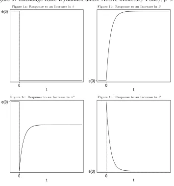
Figures 1 and 2 plot the time path of the nominal exchange depreciation rate in

re-sponse to changes ini,β,π∗ andi∗

under active and passive monetary policy, respectively.

Figure 1a shows that the rate of exchange depreciation instantaneously declines in

response to an increase in i. In this case there is no transitional dynamics, since in the

steady state a change in the nominal interest rate does not affect foreign indebtedness. The

exchange rate jumps instantaneously to the new steady state. Intuitively, an exogenous

rise in i must crowd out the endogenous component of the domestic real interest rate

(ρ(π)−π), in order to restore both the risk-adjusted interest rate parity and the PPP.

Since monetary policy overreacts to inflation, the endogenous component of the domestic

real interest rate decreases only when the rate of exchange depreciation decreases.

On the other hand, an increase in the rate of time preference β increases the level

of indebtedness and hence the cost of external borrowing. In this case, the combination

of the active Taylor rule with the risk-corrected interest parity and the PPP implies an

increase in the depreciation rate of the domestic currency. The exchange rate, in fact,

starts to increase converging gradually to its long-run equilibrium (see Figure 1b).

An increase in foreign inflation π∗

causes external indebtedness to raise and the rate

of exchange depreciation to fall in the long run, as it emerges from equations (34) and

(35). Under an active monetary policy, a rise in foreign inflation implies a reduction on

impact of the domestic currency depreciation rate, which overshoots its long-run value

asymptotically a new steady-state below its original level.

Figure 1d shows that an increase in the world interest rate i∗

determines an upward

jump of the rate of exchange depreciation on impact, since foreign bonds become more

attractive. This implies a decline in the steady-state foreign debt, as it emerges from

(34). As long as the monetary authorities are engaged in an active interest rate policy,

the reduction in the level of external debt over time must be associated with a decline in

e, along the adjustment path towards the new steady-state equilibrium. This can occur

if only if there is an instantaneous upward jump in e.

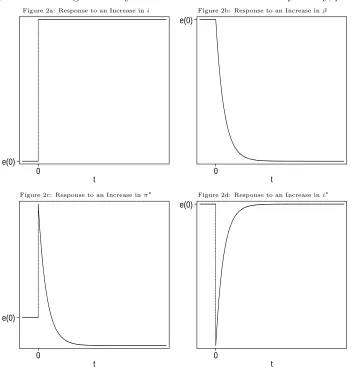
From Figures 2a-2d, one can see how the responses of the nominal exchange rate

obtained under an interest rate rule satisfying the Taylor principle are reversed in the

case of an accommodating monetary policy, underreacting to inflation. A passive Taylor

rule requires a decline in the exchange depreciation rate each time that a domestic real

interest rate increase is necessary to restore the equilibrium due, for example, to increases

inβ ori∗

(see Figures 2b and 2d). On the other hand, an increase inirequires a reduction

in the endogenous component of the domestic real rate implying, under a passive rule, a

higher depreciation rate (see Figure 2a). An increase in foreign inflation requires a

long-run fall in the rate of exchange depreciation, although it brings about an upward jump of

e on impact (see Figure 2c). In this case, only the short-run response crucially depends

on the monetary policy regime, while the effects of the PPP prevail in the long run.

7

Optimal Monetary Policy

We now derive the implications for the optimal design of interest rate policies. The

op-timizing problem for the central bank is to choose the monetary-policy responsiveness to

inflation, i.e., ρ′

,in order to maximize the representative consumer’s lifetime utility

func-tion (5) given the following perfect-foresight equilibrium solufunc-tions describing the perfectly

f) (see Appendix C):

c=c− cµσ

′

µ λ

¡

f0−f

¢

eλt, (41)

ℓ =ℓ− ℓµσ

′

µ λ

¡

f0−f

¢

eλt, (42)

m=m+

µ _ρ′

ηf ρ′₋

1−

mµσ

′

µ λ

¶ ¡

f0−f

¢

eλt_{. (43)}

Consistently with Friedman (1969), let us suppose that the function V (•) is strictly

increasing in real money balances as long as m < ms_{, but not increasing for m > m}s_,

where ms _{> m¯ represents a finite level of real money balances at which consumers are}

satisfied with liquidity.2 _{Specifically, let us assume a sufficiently high satiation level m}s_,

such that ms _{>m¯ +}³_η f −

mµσ′µ

λ ´

¡

f0−f

¢

eλt_{. Optimality must imply that}

ρ′

= 0 if f0 > f , (44)

1< ρ′

< 1

1− _ms 1

−m ηf(f0−f)eλt+

mµσ′µ ηf λ

if f0 < f . (45)

According to (44) and (45), the optimal degree of reactiveness of the nominal interest rate

to inflation critically depends on the level foreign debt. In particular, if the outstanding

foreign debt is above its steady-state target level, i.e., f0 > f, it is optimal to adopt a

fully accommodating monetary policy, ρ′

= 0. By contrast, if the outstanding foreign

debt is below its steady-state target level, i.e.,f0 < f, it is optimal to adopt an aggressive

monetary policy, satisfying the Taylor principleρ′

>1.

The economic interpretation for these findings goes as follows. Consider first the case

in which f0 > f. According to equation (38), if the monetary authority uses a feedback

policy rule satisfying the Taylor principle,ρ′

>1, the exchange depreciation rate must be

higher than its steady-state level. According to the PPP condition, the inflation rate must

also be higher than its steady-state level. Hence the Taylor rule prescribes an increase

2

in the nominal interest rate, which lowers real money balances and so welfare. Monetary

policy should thus be fully passive in order to avoid a crowding out effect on real balances.

Note that this is result is robust to changes in the degree of elasticity of the upward-sloping

schedule of foreign debt, measured by the parameterσ′ .3

Next, consider the case in which f0 < f. According to equation (38), under an active

monetary policy stance, the exchange depreciation rate, the inflation rate and the domestic

nominal interest rate are now lower than their steady-state levels. As a result, real money

balances and so welfare increase. Note that in this case, an increase in the elasticity of the

schedule of foreign debt requires a less active monetary policy stance. This is because the

higherσ′

, i.e., the more elastic the schedule of foreign debt, the higherη_f, i.e., the higher

the negative sensitivity of real balances to the differencef−f0 through the international

parity conditions, the lower the optimal value of ρ′

, i.e., the less aggressive interest rate

policies must be.

8

Concluding Remarks

External indebtedness poses constraints on the borrowing opportunities of emerging

mar-ket and developing economies, as empirically evidenced. We have analyzed the dynamic

effects of interest rate rules in the spirit of Taylor (1993, 1999) in an optimizing model of

exchange rate determination that incorporates a risk premium on foreign debt.

An imperfect global capital market has strong implications for the design of monetary

policy rules in emerging market economies that do not choose to adopt a ‘hard’ peg

exchange rate regime. In particular, it is demonstrated that when external borrowing

is subject to credit risk, the usual requirement that the monetary authorities should

fight inflation aggressively by raising the nominal interest rate more than proportionally

with respect to increases in inflation is not necessary to ensure equilibrium stability and

3

uniqueness. Under a passive monetary policy, a rise in inflation causes an increase in

private consumption, which tends to stimulate foreign borrowing. If the schedule of

external debt is upward sloping, the accumulation of foreign debt will lead to an increase

in the risk premium, which in turn will tend to reduce aggregate demand and inflation.

Thus, in the presence of external financial frictions, a non-aggressive monetary policy does

not necessarily lead to self-fulfilling inflation expectations.

On the other hand, our analytical findings show that the dynamics of exchange rates,

when the central bank implements interest rate policies, are critically affected by whether

monetary policy overreacts or underreacts to inflation. A worsening in external

indebt-edness generates an increase in the country-specific risk premium, thereby causing an

increase in the nominal interest rate faced by the small open economy. Because of the

risk-adjusted interest rate parity condition, there must be an increase in the domestic

nominal interest rate net of domestic currency depreciation. Because of the PPP

condi-tion, there must also be an increase in the domestic real interest rate. The central point

is that under an active (passive) monetary policy stance, an increase in the domestic real

interest rate does occur if and only the exchange depreciation rate increases (decreases).

Exchange rate dynamics are therefore influenced by whether the interest-rate feedback

policy rule is active or passive. In this respect, the present paper adds interesting insights

to the classical theoretical debate on exchange rate determination.

The issue of optimal monetary policy is also investigated. Should central banks in

emerging market economies take into account external indebtedness in the design of

optimal monetary rules? Should interest-rate feedback rules active or passive? Our

anal-ysis proves that the monetary-policy feedback parameter in response to an increase in

the inflation rate should crucially depend upon the outstanding level of foreign debt. In

particular, we find that it is optimal to adopt a more passive interest rate policy the

higher stock of debt denominated in foreign currency. These results cast doubts on the

interest rate rule reacting aggressively to inflation pressures.

Of course, the analysis presented in this paper is based on a number of simplifying

assumptions necessary to yield a framework by which to study the influence of external

financial frictions on monetary policy design in a quite straightforward way. Nevertheless,

at least two possible extensions are worth to be mentioned.

First, the assumption of flexible prices is primarily made for expositional simplicity.

Under sticky prices, the implied sluggish adjustment of both nominal and real variables

in response to monetary disturbances does not affect the character of our analysis in any

essential way. Second, an upward-sloping schedule of foreign debt could be derived from

explicit microfoundations. Incorporating this feature within a dynamic general

equilib-rium model is a very challenging issue. A formal analysis is beyond the scope of the

present paper. Investigation of these issues is left to future research.

References

Ag´enor, P.R. and P.J. Montiel (1999),Development Macroeconomics, Prin-ceton and

Oxford: Princeton University Press.

Bardhan, P.K. (1967), ‘Optimum Foreign Borrowing’ in K. Shell (Ed.), Essays on the

Theory of Optimal Economic Growth, Cambridge (MA): The MIT Press.

Benhabib, J., S. Schmitt-Groh´e and M. Uribe (2001), ‘Monetary Policy and Multiple

Equilibria’,American Economic Review, 91, 167-186.

Benigno, G. and P. Benigno (2008), ‘Exchange Rate Determination under Interest

Rate Rules’, Journal of International Money and Finance, 27, 971-993.

Bhandari, J.S., N.U. Haque and S.J. Turnovsky (1990), ‘Growth, External Debt, and

Sovereign Risk in a Small Open Economy’, IMF Staff Papers, 37, 388-417.

Carlstrom, C.T. and T.S. Fuerst (2001), ‘Timing and Real Indeterminacy in Monetary

De Paoli, B. (2009), ‘Monetary Policy under Alternative Asset Market Structures: The

Case of a Small Open Economy’, Journal of Money, Credit and Banking, 41, 1301-1330.

Devereux, M.B., P.R. Lane and J. Xu (2006), ‘Exchange Rates and Monetary Policy

in Emerging Market Economies’, Economic Journal, 116, 478-506.

Fischer, S. (2001), ‘Exchange Rate Regimes: Is the Bipolar View Correct?’, Journal

of Economic Perspectives, 15, 3-24.

Frankel, J.A. (1983), ‘Monetary and Portfolio-Balance Models of Exchange Rate

De-termination’, in J.S. Bhandari and B.H. Putnampp (Ed.), Economic Interdependence and

Flexible Exchange Rates, Cambridge: MIT Press.

Frenkel, J.A. (1976), ‘A Monetary Approach to the Exchange Rate: Doctrinal Aspects

and Empirical Evidence’, Scandinavian Journal of Economics, 78, 169-191.

Friedman, M. (1969), ‘The Optimal Quantity of Money’, in M. Friedman (Ed.), The

Optimal Quantity of Money and Other Essays, Chicago: Aldine.

Gal´ı, J. (2008): Monetary Policy, Inflation, and the Business Cycle, Princeton and

Oxford: Princeton University Press.

Gal´ı, J. and T. Monacelli (2005), ‘Monetary Policy and Exchange Rate Volatility in a

Small Open Economy’, Review of Economic Studies, 72, 707-734.

King, R.G. (2000), ‘The New IS-LM Model: Language, Logic, and Limits’, Federal

Reserve Bank of RichmondEconomic Quarterly, 86, 45-103.

Laxton, D. and P. Pesenti (2003), ‘Monetary Rules for Small, Open, Emerging Economies’,

Journal of Monetary Economics, 50, 1109-1146.

Leeper, E.M. (1991), ‘Equilibria under ‘Active’ and ‘Passive’ Monetary and Fiscal

Policy’, Journal of Monetary Economics, 27, 129-147.

McCallum, B.T. (1990), ‘Inflation: Theory and Evidence’, in B.M. Friedman and F.H.

Hahn (Ed.), Handbook of Monetary Economics, Amsterdam: North-Holland.

McCallum, B.T. (2003), ‘Multiple-Solution Indeterminacies in Monetary Policy

Montiel, P.J. (2003), Macroeconomics in Emerging Markets, Cambridge: Cambridge

University Press.

Mussa, M. (1976), ‘The Exchange Rate, the Balance of Payments, and Monetary and

Fiscal Policy under a Regime of Controlled Floating’,Scandinavian Journal of Economics,

78, 229-248.

Obstfeld, M. (1982), ‘Aggregate Spending and the Terms of Trade: Is There a

Laursen-Metzler Effect?’,Quarterly Journal of Economics, 97, 251-270.

Obstfeld, M. and K. Rogoff (1995), ‘Exchange Rate Dynamics Redux’, Journal of

Political Economy, 103, 624-660.

Taylor, J.B. (1993), ‘Discretion Versus Policy Rules in Practice’, Carnegie-Rochester

Conference Series on Public Policy, 39, 195-214.

Taylor, J.B. (1999), Monetary Policy Rules, Chicago and London: University of

Chicago Press.

Taylor, J.B. (2001), ‘Using Monetary Policy Rules in Emerging Market Economies’,

in Stabilization and Monetary Policy: The International Experience, Mexico City: Bank

of Mexico, 441-458.

Turnovsky, S.J. (1997), International Macroeconomic Dynamics, Cambridge (MA):

The MIT Press.

Woodford, M. (1990), ‘The Optimal Quantity of Money’, in B.M. Friedman and F.H.

Hahn (Ed.), Handbook of Monetary Economics, Amsterdam: North-Holland.

Woodford, M. (2003),Interest and Prices, Princeton and Oxford: Princeton University

Appendix A

Consumption and labor supply can be expressed as function ofµand Λ as follows. Totally

differentiate (7) and (8), given Λφ′

(ℓ) =w, and write the results in matrix notation:



 

Ucc Ucℓ

Uℓc Uℓℓ+ Λφ

′′ µ       dc dℓ   =    1 0

−Λφ′

−φ′

µ       dµ dΛ  

. (A1)

Let Ψ≡Ucc(Uℓℓ + Λφ

′′

µ)−U2

cℓ>0. We obtain the following results:

cµ= dc dµ = ¯ ¯ ¯ ¯ ¯ ¯ ¯

1 Ucℓ

−Λφ′

Uℓℓ+ Λφ

′′ µ ¯ ¯ ¯ ¯ ¯ ¯ ¯ Ψ =

Uℓℓ+ Λφ

′′

µ+UcℓΛφ

′

Ψ <0, (A2)

cΛ=

dc

dΛ =

¯ ¯ ¯ ¯ ¯ ¯ ¯

0 Ucℓ

−φ′

µ Uℓℓ+ Λφ

′′ µ ¯ ¯ ¯ ¯ ¯ ¯ ¯ Ψ =

Ucℓφ

′

µ

Ψ <0, (A3)

ℓµ= dℓ dµ = ¯ ¯ ¯ ¯ ¯ ¯ ¯

Ucc 1

Uℓc −Λφ

′ ¯ ¯ ¯ ¯ ¯ ¯ ¯

Ψ =−

UccΛφ

′ +Uℓc

Ψ >0, (A4)

ℓΛ =

dℓ

dΛ =

¯ ¯ ¯ ¯ ¯ ¯ ¯

Ucc 0

Uℓc −φ

′ µ ¯ ¯ ¯ ¯ ¯ ¯ ¯

Ψ =−

Uccφ

′

µ

Ψ >0. (A5)

Consider now the derivation of the exchange rate determination function (24). By

combining equations (2)-(4) with the Taylor rule (16), we obtain:

i∗

+σ(f) +e=i+ρ(π∗

Totally differentiating the above expression gives:

de(ρ′

−1) =di∗ +σ′

df −di+ρ′

dπ∗

. (A7)

Letting de di∗ (ρ

′

−1) =ǫi∗ = 1,de_df (ρ

′

−1) =ǫf =σ′,de_di(ρ′−1) = ǫi =−1 and _dde

π∗ (ρ

′

−1) =

ǫπ∗ =−ρ′, equation (24) immediately follows.

Finally, the equation describing the time path of real money balances can be obtained

by combining (9) with the Taylor rule (16):

V′

(m) =µ(i+ρ(π∗

+e)). (A8)

Totally differentiating yields:

V′′

dm=Rdµ+µ(di+ρ′

dπ∗ +ρ′

de), (A9)

which, given (A7), can be re-written as:

dm = R

V′′dµ+ 1

ρ′₋₁

ρ′

σ′

df −di−ρ′

dπ∗ +ρ′

di∗

V′′ µ. (A10)

Letting dm_dµ =mµ= _VR′′, dm di∗

ρ′−1

ρ′ =ηi∗ = µ V′′,

dm df

ρ′−1

ρ′ =ηf = σ′_µ V′′,

dm di

ρ′−1

ρ′ =ηi =− µ ρ′_V′′ and dm

dπ∗ ρ′−₁

ρ′ =ηπ∗ =− µ

Appendix B

Totally differentiate (25) and (26) and express the results in matrix notation:



 

0 σ′

cµ(µ,Λ)−Λφ

′

ℓµ(µ,Λ) β       dµ df   =   

1 0 0 1 −1

−f κ −1 0 0

               dβ dΛ dg dπ∗ di∗             ,

where κ≡φ(ℓ(µ,Λ)) + Λφ′

ℓΛ(µ,Λ)−cΛ(µ,Λ)>0.

Letting ∆ ≡ −σ′

(cµ(µ,Λ)−Λφ

′

ℓµ(µ,Λ)) > 0 we obtain the following set of

deriva-tives: dµ dβ = ¯ ¯ ¯ ¯ ¯ ¯ ¯ 1 −f σ′ β ¯ ¯ ¯ ¯ ¯ ¯ ¯ ∆ =

β+σ′

f

∆ >0, (B1)

dµ

dΛ =

¯ ¯ ¯ ¯ ¯ ¯ ¯ 0 κ σ′ −β ¯ ¯ ¯ ¯ ¯ ¯ ¯ ∆ =− κσ′

∆ <0, (B2)

dµ dg = ¯ ¯ ¯ ¯ ¯ ¯ ¯ 0 −1 σ′ β ¯ ¯ ¯ ¯ ¯ ¯ ¯ ∆ = σ′

∆ >0, (B3)

dµ dπ∗ =

¯ ¯ ¯ ¯ ¯ ¯ ¯ 1 0 σ′ β ¯ ¯ ¯ ¯ ¯ ¯ ¯ ∆ = β

∆ >0, (B4)

dµ di∗ =

¯ ¯ ¯ ¯ ¯ ¯ ¯ −1 0 σ′ β ¯ ¯ ¯ ¯ ¯ ¯ ¯ ∆ =− β

df dβ = ¯ ¯ ¯ ¯ ¯ ¯ ¯ 0

[cµ(µ,Λ)−Λφ

′

ℓµ(µ,Λ)]

1 −f ¯ ¯ ¯ ¯ ¯ ¯ ¯ ∆ =−

cµ(µ,Λ)−Λφ

′

ℓµ(µ,Λ)

∆ =

1

σ′ >0, (B6)

df

dΛ =

¯ ¯ ¯ ¯ ¯ ¯ ¯ 0

cµ(µ,Λ)−Λφ

′

ℓµ(µ,Λ)

0 κ ¯ ¯ ¯ ¯ ¯ ¯ ¯

∆ = 0, (B7)

df dg = ¯ ¯ ¯ ¯ ¯ ¯ ¯ 0

cµ(µ,Λ)−Λφ

′

ℓµ(µ,Λ)

0 −1 ¯ ¯ ¯ ¯ ¯ ¯ ¯

∆ = 0, (B8)

df dπ∗ =

¯ ¯ ¯ ¯ ¯ ¯ ¯ 0

cµ(µ,Λ)−Λφ

′

ℓµ(µ,Λ)

1 0 ¯ ¯ ¯ ¯ ¯ ¯ ¯ ∆ =−

cµ(µ,Λ)−Λφ

′

ℓµ(µ,Λ)

∆ =

1

σ′ >0, (B9)

df di∗ =

¯ ¯ ¯ ¯ ¯ ¯ ¯ 0

cµ(µ,Λ)−Λφ

′

ℓµ(µ,Λ)

−1 0 ¯ ¯ ¯ ¯ ¯ ¯ ¯ ∆ =

cµ(µ,Λ)−Λφ

′

ℓµ(µ,Λ)

∆ =−

1

σ′ <0. (B10)

Given the above results and using (21)-(24), one obtains the long-run effects on

consump-tion, labor inputs, income, real money balances and exchange rates. This shows results

reported in Tables 1 and 2.

Appendix C

Focusing on the stable path, the solutions for µ, f, c, ℓ, y, m and e are of the following

form:

µ=µ− σ

′

µ λ

¡

f0−f

¢

eλt, (C1)

f =f +¡

f0−f

¢

eλt, (C2)

ℓ=ℓ+ℓµ(µ−µ), (C4)

y =y+φ′

ℓµ(µ−µ), (C5)

m=m+mµ(µ−µ) + ρ′

ρ′

−1ηf

¡

f−f¢

, (C6)

e=e+ 1

ρ′₋₁ǫf

¡

f −f¢

, (C7)

where λ <0 is the stable eigenvalue andf0 is the initial condition on foreign debt.

Appendix D

At time t = 0, differentiating (C1)-(C7) with respect to some arbitrary variable, say x,

yields:

dµ(0)+

dx = dµ dx + σ′ µ λ df

dx, (D1)

df(0)+

dx = 0, (D2)

dc(0)+

dx =

dc dx +cµ

µ dµ(0) dx − dµ dx ¶ , (D3)

dℓ(0)+

dx =

dℓ dx +ℓµ

µ dµ(0) dx − dµ dx ¶ , (D4)

dy(0)+

dx =

dy

dx +φ

′ ℓµ µ dµ(0) dx − dµ dx ¶ , (D5)

dm(0)+

dx =

dm

dx +mµ

µ dµ(0) dx − dµ dx ¶ − ρ ′ ρ′

−1ηf

df

dx, (D6)

de(0)+

dx =

de

dx −

σ′

ρ′₋ 1

df

dx. (D7)

From the above relationships for x =i, β,Λ, g, i, π∗

, using the results reported in Tables

Table 1: Steady-State Effects of Changes in Domestic Variables and Parameters

i β Λ g

µ 0 β+σ′_f

∆ >0 −

[φ(ℓ)+Λφ′_ℓ Λ−cΛ]σ′

∆ <0

σ′

∆ >0

f 0 1

σ′ >0 0 0

c 0 cµβ+σ

′_f

∆ <0 cΛ−

[φ(ℓ)+Λφ′_ℓ

Λ−cΛ]σ′cµ

∆ >0

σ′_cµ

∆ <0

ℓ 0 ℓµβ+σ

′_f

∆ >0 ℓΛ−

[φ(ℓ)+Λφ′_ℓ

Λ−cΛ]σ′ℓµ

∆ ⋚0

σ′_ℓ

µ

∆ >0

y 0 φ′

ℓµβ+σ ′_f

∆ >0 φ

′

ℓΛ− [

φ(ℓ)+Λφ′_ℓ

Λ−cΛ]σ′φ′ℓµ

∆ ⋚0

σ′_φ′_ℓ

µ

∆ >0

m −_Vµ′′

1

ρ′−1 ≷0

R V′′

β+σ′_f

∆ +

µ V′′_(ρ′−1)ρ

′ ≶

0 −[φ(ℓ)+Λφ

′_ℓ Λ−cΛ]σ′

∆

R V′′ >0

σ′

∆

R V′′ <0

e −_ρ′1−1 ≶0

1

ρ′−1 ≷0 0 0

Table 2: Steady-State Effects of Changes in Foreign Variables

π∗

i∗

µ _∆β >0 −_∆β <0

f 1

σ′ >0 −

1

σ′ <0

c −cµ_∆β <0 cµ_∆β >0

ℓ −ℓµ_∆β >0 ℓµ_∆β <0

y −φ′

ℓµ_∆β >0 φ

′

ℓµ_∆β <0

m _VR′′

β

∆ <0 −

R V′′

β

∆ >0

Table 3: Impact Effects of Changes in Domestic Variables and Parameters

i β Λ g

µ(0)+ 0 dµ

dβ − µ λ1 >0

dµ dΛ <0

dµ dg >0

c(0)+ 0 dc

dβ −cµ µ λ1 <0

dc dΛ T0

dc dg <0

ℓ(0)+ 0 dℓ

dβ − µ

λ1ℓµ>0

dℓ dΛ S0

dℓ dg >0

y(0)+ 0 dy_dβ −_λµ

1φ

′

ℓµ>0 _ddy_Λ S0 dy_dg >0

m(0)+ −_Vµ′′

1

ρ′−₁ ≷0

R V′′

β+σ′_f

∆ −

R V′′

µ

λ1 <0 −

[φ(ℓ)+φ′_ℓ Λ−cΛ]σ′

∆

R V′′ >0

σ′

∆

R V′′ <0

e(0)+ −_ρ′1−1 ≶0 0 0 0

Table 4: Impact Effects of Changes in Foreign Variables

π∗

i∗

µ(0)+ _dπdµ∗ −

µ λ1 >0

dµ di∗ +

µ λ1 <0

c(0)+ dc

dπ∗ −cµ µ λ1 <0

dc di∗ +cµ

µ λ1 >0

ℓ(0)+ dℓ

dπ∗ −ℓµ µ λ1 >0

dℓ di∗ +ℓµ

µ λ1 <0

y(0)+ _dπdy∗ −φ

′

ℓµ_λµ₁ >0 _didy∗ +φ

′

ℓµ_λµ₁ <0

m(0)+ _V1′′ ³

βR

∆ −

Rµ λ1 −

ρ′_µ ρ′−₁

´

≷0 _V1′′ ³

−βR_∆ +Rµ_λ

1 +

ρ′_µ ρ′−₁

´

≶0

e(0)+ −_ρ′1−1ρ

′ ≶

Figure 1: Exchange Rate Dynamics under Active Monetary Policy, ρ′

>1

Figure 1a: Response to an Increase ini Figure 1b: Response to an Increase inβ

e(0)

0

t

e(0) 0

t

Figure 1c: Response to an Increase inπ∗ Figure 1d: Response to an Increase ini∗

e(0)

0

t

e(0) 0

Figure 2: Exchange Rate Dynamics under Passive Monetary Policy, ρ′

<1

Figure 2a: Response to an Increase ini Figure 2b: Response to an Increase inβ

e(0) 0

t

e(0)

0

t

Figure 2c: Response to an Increase inπ∗ Figure 2d: Response to an Increase ini∗

e(0)

0

t

e(0)

0