Confounding of Three Binary-Variable Counterfactual
Model with DAG
Jingwei Liu, Shuang Hu
School of Mathematics and System Sciences, Beihang University, Beijing, China Email: [email protected]
Received May 30, 2013; revised June 30, 2013; accepted July 7, 2013
Copyright © 2013 Jingwei Liu, Shuang Hu. This is an open access article distributed under the Creative Commons Attribution Li-cense, which permits unrestricted use, distribution, and reproduction in any medium, provided the original work is properly cited.
ABSTRACT
Confounding of three binary-variable counterfactual model with directed acyclic graph (DAG) is discussed in this paper. According to the effect between the control variable and the covariate variable, we investigate three causal counterfac-tual models: the control variable is independent of the covariate variable, the control variable has the effect on the co-variate variable and the coco-variate variable affects the control variable. Using the ancillary information based on condi-tional independence hypotheses and ignorability, the sufficient conditions to determine whether the covariate variable is an irrelevant factor or whether there is no confounding in each counterfactual model are obtained.
Keywords: Causal Effect; Independence Hypothesis; Counterfactual Model; Confounding Bias; Irrelevant; Ancillary Information; Directed Acyclic Graph
1. Introduction
Causal inference has become an important research field in statistics, data mining, epidemiology and machine learn-ing etc. in recent decades [1-7], and directed acyclic graph (DAG) is involved in describing the relationship between causal connections [4]. Confounding and con-founder are two basic concepts for epidemiology causal inference [1,3]. Several models have been presented for causal inference, two of which are the causal diagram model and counterfactual model [6,8,9].
To assess confounding and confounder, two main ap-proaches, “collapsibility-based” and “comparability-based”, are discussed in [10], which regard confounding bias as arising from differences between stratified measures of association and the corresponding original measure or from the exposed and unexposed populations which are not comparable. The comparability-based approach de-termines a factor to be a confounder if adjusting for it can reduce confounding bias [3,10]. Geng etal. (2002) [11] point out that the effect of exposure on the rate of a dis-ease cannot be assessed correctly in the presence of founding bias. They propose probability criteria for con-founding and discuss concon-founding with multi-value co-variate variables. However, their work does not clearly analyze general causal DAG even with three binary- variables, since the simple case of their definition about covariate can only be expressed by Figure 1 (see Figure
6.2 in p. 61, [12]).
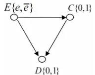
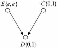
[image:1.595.374.472.536.618.2]As to three binary-variable DAGs, [5,13] discussed identifiability of the causal effect of the other two kinds of counterfactual models (Figures 2 and 3) using the inde-pendence hypotheses respectively. Yet, the confounding and confounder in these two simple causal DAGs are not discussed explicitly. For Figure 2 (see Figure 6.5 in p. 64, [12]), the covariate C is an intermediate variable in the causal chain. [6,12] (p. 30) discuss the intermediate vari-able causal chain, however more varivari-ables are involved
Figure 1. The first model.
[image:1.595.375.471.642.718.2]Figure 3. The third model.
in fitting “Back-door” formula and “Front-door” formula. Traditionally, a confounding variable (the precise defi-nition of a confounder) is a variable which is a common cause of both the control variable and the response vari-able [14] (see Figure 1). Whether the covariate varivari-able, which is not a common cause of both the control variable and the response variable in three binary-variable coun-terfactual models, is a confounder? [1,10] develop a qualitative definition of confounder: controlling a vari-able can reduce confounding, then the varivari-able is called a confounder. Hence, the covariate variable, which is not a common cause of both the control variable and the re-sponse variable, but affects the rere-sponse variable, may be a confounder. Recently, the confounder and confounding detection attracts more attention in gene network discov-ery [15], the question arises from how to investigate the causal DAG in a pure gene network and how to analyze the role of covariate from statistical data if we think that there is causation structure in gene network? It is neces-sary to discuss the confounder and confounding in the general causal DAG diagram. These motivations drive us to investigate the confounding and confounder in general causal DAG with the definitions in [11].
In this paper, according to the precise definition, one model as shown in Figure 1 is discussed: the covariate variable affects the control variable and the response variable at the same time, and the control variable affects the response variable. By the qualitative definition, we investigate other two models: one, as shown in Figure 2, is that the control variable has the effect on the covariate variable and the covariate variable affects the response variable; the other, as shown in Figure 3, is that the con-trol variable is independent to the covariate variable and the covariate variable affects the response variable. Ob-viously, the third model is the special case of the other two models with independence of the control variable and the covariate variable. Then we use the formal defi-nitions of a confounder and an irrelevant factor in [11] and the ancillary information based on conditional inde-pendence hypotheses [5,13] to discuss the confounding of above-mentioned counterfactual models.
The rest of the paper is organized as follows: In Sec-tion 2, we introduce the main notaSec-tion and definiSec-tions, and discuss the relationship between confounder and
ir-relevant factor. In Section 3, confounding and irir-relevant factor of three kinds of three binary-variable counterfac-tual models with DAGs are discussed respectively. The conclusion is given in Section 4.
2. Notation and Definitions
Let E, D, C be binary variables. Let the control variable
E be an exposure with the values e and e represent-ing “exposed” and “unexposed” respectively. Let the response variable be an outcome with the values 0 and 1 denoting the presence or absence of a disease, where e is the corresponding response when
D
D Ee
and De is the corresponding response when Ee,
both of which take values 1 or 0 denoting the presence or absence of a disease. Let be a covariate variable with possible values 0 or 1.
C
Many kinds of studies focus on the effects of exposure on the rate of a disease in the exposed population. Let
e 1
P D Ee and P D
e1Ee
be the propor-tions of diseased individuals in the unexposed population and the exposed population. Let P D
e 1Ee
be the hypothetical proportion of individuals in the exposed population who would have attacked by the disease even if they had not been exposed. Since P D
e 1Ee
is a hypothetical proportion, the model is a counterfactual model [8,9].In order to identify the casual effect of exposure on response, confounding bias is defined as the differ-ence between the hypothetical proportion of diseased individuals in the exposed population [16,17], that is
B
e 1
e 1BP D E e P D Ee
(2.1) If B0, then there is no confounding.By the common standardization in epidemiology [1,2, 11,18-20], the standardized proportion P D
e 1Ee
,which is obtained by adjusting the distribution of in the unexposed population to that in the exposed popula-tion, is
C
1
0
1
1 e
e k
P D E e
P D E e C k P C k E e
(2.2)
Definition 1 [11]. A covariate C is a confounder if
e 1
e 1
P D E e P D Ee B (2.3) From the definition, we find that the standardized proportion P D
e1Ee
obtained by adjusting for the irrelevant factor is closer to the hypothetical pro-portion P D
e 1Ee
than the observed proportion
e 1
P D Ee .
Definition 2 [11]. A covariate is an irrelevant factor if
e 1
e 1
P D Ee P D Ee (2.4)
Since the estimation of the hypothetical proportion is still unchanged after being adjusted for an irrelevant fac-tor, we do not need to adjust it to reduce confounding bias. And, the relationship between irrelevant factor and confounder is obtained in Lemma 1:
Lemma 1. If a covariate is an irrelevant factor, it is not a confounder. Inversely, if is a confounder, it is not an irrelevant factor.
C C
Proof.
According to the condition that C is an irrelevant factor, we can obtain that
e 1
e 1
P D Ee P D Ee Then,
1 1
1 1
e e
e e
P D E e P D E e
P D E e P D E e B
which means C is not a confounder.
From the condition that is a confounder, we can obtain
C
1 1
1 1
e e
e e
P D E e P D E e
B P D E e P D E e
Then,
e 1
e 1
P D Ee P D Ee
In fact, if
e 1
e 1
P D Ee P D Ee , Then,
1 1
1 1
e e
e e
P D E e P D E e
P D E e P D E e B
This is a contradiction!
Hence, C is not an irrelevant factor. □
[11] (pp. 7-8) gives an example, and illustrates two cases of irrelevant factor and confounder respectively. To illuminate conceptions of confounding and irrelevant factor and Lemma 1, we continue to discuss the relation-ship based on their original example and give two exam-ples as follows.
Example 1. For example in [11]. Let a factor ex-press groups categorized by every 10 years of age, and its values 1, 2, 3 and 4 denote the original age groups 20 - 29, 30 - 39, 40 - 49 and 50 - 59 years respectively, we denote it as
C
1 , 2 , 3 , 4
. Suppose that there is no exposure effect, i.e. there are only individuals of type 1 (individual ’doomed’) and type 4 (individual immune to disease), and that the joint distribution of disease,ex-posure and a factor is given in Table 1 of [11] (p. 7), where
C
1 0
1 0
0 06
e
e
P D E e
P D E e
B
52
58
When the individuals are regrouped by “younger than 50”, we denote it as p
1, 2,3 , 4
, which means we adjust the distribution of C, a coarse subpopulation is given in Table 1.Then,
1
122 250 52 50 200 300 100 300
0 595 0 58 1
p e
e
P D E e
P D E e
And,
1
1
0 595 0 52 0 075
e p e
P D E e P D E e
B
That is, is not a confounder, and it is not an ir-relevant factor.
C
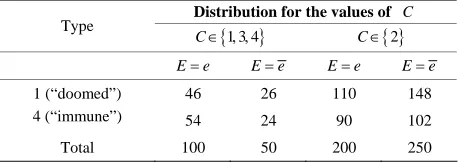
Example 2. To continue the discussion of above ex-ample in [11], when the individuals are regrouped by “younger than 40 but older than 30”, we denote it as
1,3, 4 , 2
p , we can obtain a coarse subpopulation given in Table 2.
Then,
26 100 148 200 1
50 300 250 300 0 568 0 58 1
p e
e
P D E e
P D E e
[image:3.595.309.538.539.617.2]
Table 1. Example of a factor C which is neither a con-founder, nor an irrelevant factor.
Distribution for the values of C
Type
1 2 3
C C 4
Ee Ee Ee Ee
1 (“doomed”) 133 122 23 52
4 (“immune”) 117 78 27 48
Total 250 200 50 100
Table 2. Example of a factor C which is not an irrelevant factor, but is a confounder.
Distribution for the values of C
Type
1 3 4
C C 2
Ee Ee Ee Ee
1 (“doomed”) 46 26 110 148
4 (“immune”) 54 24 90 102
[image:3.595.309.538.656.737.2]Hence,
1
1
0 568 0 52 0 048
e p e
P D E e P D E e
B
To sum up, is not an irrelevant factor, but is a confounder.
As announced in [11], regrouping C
1, 2 , 3, 4
p ,
co
C is a confounder, but not an irrelevant factor. Exam-ple 2 shows that nfounder is not unique,
1,3, 4 , 2
is another case, and
-t values of
p they have differ
en B .
Conclusion: According to Lemma 1, Example 1, Ex-ampl 11], whether a factor C is a confounder or an irrelevan actor depends on the adjusting distribu-tio
e 2 and [ t f
ow
n p
ing the confounding of three binary-variable coun-dels n of C. That is, even for a fixed factor C in a spe-cific experiment, for example, age, h to judge it as a confounder or an irrelevant factor relies on the “right” adjustme t of its distribution. And, more im ortant, the non-uniqueness of confounder makes the causal analysis be more complex.
If we transform the adjustment of covariate variable in Figure 1 to the intervention distribution in counterfactual models in Figures 2 and 3, the definition 1 and definition 2 would be easily employed in the discussion of con-founding and irrelevant factor in the other general causal DAGs.
3. Confounding of Counterfactual Model
Consider
terfactual models, there are three counterfactual mo of causal DAGs as follows (Figures 1-3):
To discuss whether there be confounding in our con-sidering models, we use the conditional independence hypotheses as follows as the ancillary information (H):
1) EDe
2) ED Ce 0
3) ED Ce 1
4) E C 5) De C
6) De C E e 7) DeC E e
3.1. The First Model
A own in Figure 1, has effect on and at the same time, and ffects . In or o ca ate
s sh C
a
E der t
D lcul
C E
simply, suppose that
101 0
0,1.
1 0
1 1
e j
e
e
C j b j
P D E e C u
P D E e C u
1 0
1
1
P C t
P E e C a P E e C a
P D E e
0 0 1 1
1 1 1 j 1 j
t t a a a a b b where t a a b 0 1 j
0 1
u u
can be observed from original data, but can not
roportions
be observed because they are
hypo-th .
Then, we obtain the following formulae, etical p
1
0
0 0 1 1
1E e C k P C k E e
a t b a t
1 e
e k
P D E e
P D
b
0 1
a t a t
1
0
0 0 1 1
0 1
1
1 e
e k
P D E e
P D E e C k P C k E e
u a t u a t
a t a t
1
0
0 0 1 1
0 1
1
1 e
e k
P D E e
P D E e C k P C k E e
b a t b a t
a t a t
And,
0 0 1 1 0 0 1 1
0 1 0 1
1 1
e e
B P D E e P D E e
b a t b a t b a t b a t a t a t a t a t
Using the above formulae, we translate each condition of o parameter form:
1) (
H
) int0 0 1 1 0 0 1 1
0 1 0 1
e
b a t b a t b a t b a t E D i e
a t a t a t a t
0 0
0
e
ED C i e u b 2)
1 1
1 e
ED C i e u b 3)
4) CD i e u ae 0 0b a0 0u a1 1b a1 1
5) CD Ee e i e b 0 b1
6) CD Ee e i e u 0 u1
7) CE i e a 0a1
Theorem 1. If one of the following conditions holds, a) EC
b) De C Ee
c) De C Ee E, D Ce
The covariate is an irrelevant factor. of.
der to prove irrelevant factor, we only ne
C Pro
In or C is an
ed to prove
0 0 1 1 0 0 1 1
0 1 0 1
b a t b a t b a t b a t a t a t a t a t
[image:4.595.317.516.151.464.2]
b0b1
a0a1
0a) From the condition EC, we can obtain
Then,
0 1
a a
e 1
e 1
P D Ee P D Ee
b) From the condition De C Ee, we can obtain
Then,
0 1
b b
e 1
e 1
P D Ee P D Ee
c) From the condition ED Ce , we can ob ain t 0
e
ED C i.e. u0b0,
1 e
ED C i.e. u1b1. Since,
0 1
e
CD Ee i e u u
Hence, We obtain,
0 1
b b
e 1
e 1
P D Ee P D Ee □ Theorem 2. If one of the following con itions holds, a)
d
e
b) ED
e
CD E e E D Ce c) ED Ce 0 C D Ee d) ED Ce 1C D Ee e) EDe C E C There is no confounding. Proof.
a) From the condition EDe, we can obtain
0 0 1 1 0 0 1 1
0 1 0 1
b a t b a t b a t b a t
a t a t a t
n,
a t
The
0 0 1 1
b a t b a t
B
0 0 1 1
0 1 0 1
0
b a t b a t a t a t a t a t
b) From the condition ED Ce , we can obtain 0
e
ED C i.e. u0b0.
1 e
ED C i.e. Furthermore,
1 1
u b
e
CD Ee i.e. b0b1. We obtain,
0 0 1 1 b a t0 0 1 1
0 1 1
0
b a t b a t b a t B
a t a t a t
0
a t
c) From the condition CD Ee , we can obtain e
CD Ee i.e. b0b1;
e
CD Ee i.e. From the other condition, we obtain
0 1
u u
i.e. u0b0.
0 e
ED C Then,
0 0 1 1 0 0t b1 1
0 0
0 1
0
b a t b a t b a a t
B u b
a t a t a t t
0 a1
d) From the condition CD Ee , we can obtain e
CD Ee i.e. b0b1,
e
CD Ee i.e.
Furthermore, according to the next condition, we have
0 1
u u .
i.e. u1b1.
1 e
ED C Then,
0 0 1 1 0 0t b1 1
1 1
0 1
0
b a t b a t b a a t
B u b
a t a t a
0t a t1
e) From the condition
e
ED C, we can obtain
0
ED Ce i.e. u0b0;
1 e
ED C i.e. u1 b1
Furthermore,
0 1
CE i e a a Then,
0 0 1 1 0 0t 0
a t
1 1
0 1 0 1
b a b
B
a t a t a t
b a t b a t a t
□
3.2. The Second Model
As shown in Figure 2, and ve effect on at the same time, and ffects r to
la pose:
E a
C C
ha . In orde
D calcu-E
te simply, sup
0
1 0
1 1
e
e
P D E e C u
P D E e u
1 0
1
1 1
j
P E e a
P C E e c P C E e c
j b
C
1
e
P D E e C
0 0 1 1
1 1 1 j 1 j
j a b
, u1
prop
where can be observed from original data. But can not be observed because they are hyp ortions, also can be treated as counterfact model by intervention [13].
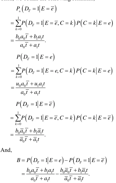
Then, we obtain the following formulae,
0 c , o-ual
1 c, thet
0 u
ical
1
0
0 1 b c1 1
1
1
e
e k
P D E e
P D E e C k P C k E e
b c
1
1 e
P D Ee
0
1 e k
P D E e C k P C k
0 1 1 1
E e
u c u c
1
0
0 0 1 0
1
1 e
e k
P D E e
P D E e C k P C k E e
b c b c
Then,
0 1 1 1 0 0 1 0
1 1
e e
B P D E e P D E e
u c u c b c b c
Using the above formulae, we translate each condition of (H) into parameter form:
1) ED i e u ce 0 1u c1 1b c0 0b c1 0
2) ED Ce 0 i e u 0b0
3) ED Ce 1 i e u 1b1
4) CDe i.e.
0 0 0 1 1 1 1 0
1 0 0 1
u c a b c a u c a b c a
c a c a c a c a
5) CD Ee e i.e. 6)
0 1
b b
e
CD Ee i.e.
ollowing conditions holds,
0 1
u u 7) CE i.e. c0c1
Theorem 3. If one of the f a) EC
b) De C Ee
c) De C E e E D Ce
The c C
Pro
ovariate is an irrelevant factor. of.
rom the condi e can obtain a) F tion EC, w
0 1
c c Then,
0 1 1 1 0 0 1 0
1
1
e
e
P D E e b c b c b c b c
P D E e
b) From the condition De C Ee, we can obtain
Then,
0 1
b b
0 1 b c11 0 1 1
0 0 0 0 1 0
1
1
e
e
P D E e b c b c c
c c b c b c P D E e
0 b
c) From the condition De C Ee, we can obtain
i.e. b0b1,
0 e
ED C
1 e
ED C i.e.
ore,
0 1
u u Furtherm
e
D C Ee i.e.
Then,
0 1
b b
e 1
P De 1E
P D Ee e □
Theorem 4. If one of the f ng con n holds, a)
ollowi ditio
e
ED
0
e e
E D C C D E
b)
c) ED Ce 1
d)
e
C D E
e
ED C E C There is no confounding.
e condition that Proof.
a) From th EDe, we can obtain
0 1 1 1 0 0 1 0
u c u c b c b c Then,
0 1 0 1 0
Bu t u tb t b t rom the condition
b) F CD Ee , we can obtain e
CD Ee i.e. b0b1,
e
CD Ee i.e. u0u1.
Furthermore,
i.e. u0b0.
0 e
ED C Then,
0 1 1 1 0 0 1 0 0 0 0
Bu c u c b c b c u b c) From the condition CDe E, we can obtain
e
CD Ee i.e. b0 b1
e
CD Ee i.e.
Furthermore,
0 1
u u .
1 e
ED C i.e.
Then,
1 1
u b .
0 1 1 1 1 1 0
Bu c u c b c0 0b c1 0 u b d) From the condition EDe C, we can obtain
i e.
0 e
ED C . u0b0, i.e. u1b1.
1 e
and, Furthermore,
i. 1.
CE e. c0c
Then,
u00 b c01
0 0
1
c0 0. 1 1
B u t u t b t b t
u t b
3.3. The Third Model
As shown in Figure 3, both E and C have effects on D, and EC.
Denote,
0
1
1
1 0
1 0
1 1
e j
e
e
P E e a P C t
P D E e C j b j
P D E e C u
P D E e C u
,1.
1 1 j 1 j
w ere
a a t t b b
h a t bj ca be obser from ginal data, but
ot or
n ved ori
be observed because they are hypothetical the probability with intervention [5]. Then,
0u1 can n
ortions,
u
prop
1
0
1
0
0 1
b t b t
1
1
1 e
e k
e k
P D E e
P D E e C k P C k E e
P D E e C k P C k
1
0
1
0
0 1
1
1 e
e k
e k
P D E e C k P C k E e
P D E e C k P C k
u t u t
1P D Ee
1
0
1
0
0 1
1
1
1
e
e k
e k
P D E e
P D E e C k P C k E e
P D E e C k P C k
b t b t
Then,
0 1 0 1
1 1
e e
B P D E e P D E e
u t u t b t b t
e 1
e 1
P D Ee P D Ee .
Hence, the covariate is an irrelevant fact but not a confounder, and it can not reduce confounding.
Using the above formulae, we translate each condition of (H) into parameter form, where is naturally
tru .
C or,
EC
e in Figure 3
1) ED i e u te 0 u t1 b t0 b t1
2) ED Ce 0 i e u 0b0
1 1
1 e
ED C i e u b
3)
0 0 1 1
e
CD i e b a u ab au a
4)
5) CD Ee e i e b 0 b1
6) CD Ee e i e u 0 u1
discussed above, in the ca
As usal DAG Figure 3 with
EC, the covariate C s naturally an irrelevant factor. To keep the same expression as other DAGs, we have
i
the fo
of Fi llowing theorem.
Theorem 5. In the causal DAG gure 3 with
EC, the covariate is an irrelevant factor. orem 5 shows that in the causal DAG Figure 3, co ate is always an irrel factor regardless of an justment or intervention on it.
eorem 6. If one of the following conditions holds,
C
The
vari C evant
y ad s
Th a) EDe
b) ED Ce 0 E D Ce 1 c) De C E E D Ce 0 b) De C E E D Ce 1 There is no confounding. Proof.
a) From the condition EDe, we can obtain
0 1 0 1
u t u tb t b t
Then,
0 1 0 1 0
Bu t u tb t b t
b) From the conditions
0 e
ED C and ED Ce 1, we can obtain
0 0
u b and u1b1.
Then,
0 1 0 1 0
Bu t u tb t b t
e condition
c) From th De C E, we can obtain
e
D C Ee i.e. b0b1,
e
CD Ee i.e.
Furthermore,
0 1
u u.
0 e
ED C i.e.
Then,
0 0
[image:7.595.61.528.123.734.2]0 1 0 1 0 0 0 Bu t u tb t b tu b
d) The proof is similar to c). □
4.
Using the formal definition confounder, non-founding and irrelevant fact discus he confound-ing of three kinds of three bi variable counterfactual m logy studies and statistics, where t general causal DAG is invo n the d scussion sufficient conditions of determ ing non-confound an nt factor in a three binary-variable causal are discussed. Our work focuses on the ge ral three
bi o other variable
in
founder and confounding are two dif-ased on probability criteria, our
dis-ion would be more complex as sh
, New York, 1982. Epidemiology,” Little Brown,
Conclusions
s of con-
or, we s t
nary-odels in epidemio he
lved i i in
. The ing DAG d irreleva
ne nary-variable causal DAG, and n
volved in discussion.
s are
Furthermore, con ferent conceptions b
cussions are definitely different from relative literatures, for example, [5,11,13]. In addition, the non-uniqueness of irrelevant factor and confounder in theory makes it more difficult to detect them and discuss the sufficient and necessary condition. The ancillary information (H) involved in our discussion is only a part of [5,13], hence we only obtain some sufficient conditions, another cause of this design lies in the thought that we want to discuss the causation along causal path. The sufficient and nec-essary condition discuss
own in our results. The future work will extend the three-variable counterfactual model to multi-variable counterfactual model. And, we will apply the theoretical results to the confounder detection in gene network.
5. Acknowledgements
This work is partially supported by National Natural Sci-ence Foundation of China for Youths (NSFC: 10801019). The author would like to thank the anonymous reviewer for the valuable comments and suggestions to make great improvement of this paper.
REFERENCES
[1] D. G. Kleinbaum, L. L. Kupper and H. Morgenstern, “Epidemiologic Research: Principle and Quantitative Me- thods,” Van Nostrand Reinhold
[2] K. J. Rothman, “Modern Boston, 1986.
[3] S. Greenland, J. M. Robins and J. Pearl, “Confounding and Collapsibility in Causal Inference,” Statistical Sci- ence, Vol. 14, No. 1, 1999, pp. 29-46.
http://dx.doi.org/10.1214/ss/1009211805
[4] J. Pearl, “Causality: Models, Reasoning and Inference,” Cambridge University Press, Cambridge, 2000.
[5] Z. G. Zheng, Y
il-ity of Causal Effect for a Simple Causal Model,” Science
ence,” 40. http://dx.doi.org/10.1360/02ys0374
in China, Vol. 45, No. 3, 2002, pp. 335-341.
[6] Z. Geng, Y. B. He and X. L. Wang, “Relationship of Causal Effects in a Causal Chain and Related Infer
Science in China Series A: Mathematics, Vol. 47, No. 5, 2004, pp. 730-7
8, pp. 459-483. f Treatments in
pp. 688- [7] X. H. Xie and Z. Geng, “A Recursive Method for
Struc-tural Learning of Directed Acyclic Graphs,” Journal of Machine Learning Research, Vol. 9, 200
[8] D. B. Rubin, “Estimating Causal Effects o
Randomized and Non Randomized Studies,” Journal of Educational Psychology, Vol. 66, No. 5, 1974,
701. http://dx.doi.org/10.1037/h0037350
[9] P. W. Holland, “Statistics and Causal Inference,” Journal of the American Statistical Association, Vol. 81, No. 396, 1986, pp. 945-970.
http://dx.doi.org/10.1080/01621459.1986.10478354 [10] S. Greenland and J. M. Robins, “Identifiability Exchange-
ability and Epidemiologic Confounding,” International Journal of Epidemiology, Vol. 15, No. 3, 1986, pp. 413- 419. http://dx.doi.org/10.1093/ije/15.3.413
[11] Z. Geng, J. H. Guo and W. K. Fung, “Criteria for Con- founders in Epidemiological Studies,” Journal of the Royal Statistical Society: Series B (Statistical Methodol- ogy), Vol. 64, No. 1, 2002, pp. 3-15.
http://dx.doi.org/10.1111/1467-9868.00321
[12] C. Berzuini, P. Dawid and L. Bernardinelli, “Causality: Statistical Perspectives and Applications,” John Wiley & Sons, Hoboken, 2012.
http://dx.doi.org/10.1002/9781119945710
[13] Y. Liang and Z. G. Zheng, “The Identifiability Condition of Causal Effect for a Simple Causal Model,” Acta Ma- thematica Scientia, Vol. 23A, No. 4, 2003, pp. 456-463. [14] G. Wunsch, “Confounding and Control,” Demographic
Research, Vol. 16, No. 4, 2007, pp. 97-120. http://dx.doi.org/10.4054/DemRes.2007.16.4
[15] J. E. Aten, “Causal Not Confounded Gene Networks: Inferring Acyclic and Non-acyclic G
works in mRNA Expression Studies using
ene Bayesian Net-Recursive V-
onfounding in Structures, Genetic Variation, and Orthogonal Causal Anchor Structural Equation Models,” Ph.D. Dissertation, University of California, Oakland, 2008.
[16] P. J. Wickramaratne and T. R. Holford, “C
Epidemiologic Studies: The Adequacy of the Control Groups as a Measure of Confounding,” Biometrics, Vol. 43, No. 4, 1987, pp. 751-765.
http://dx.doi.org/10.2307/2531530
[17] P. W. Holland, “Reader Reactions: Confounding in Epi- demiologic Studies,” Biometrics, Vol. 45, No.
1310-1316.
. Y. Zhang and X. W. Tong, “Identifiab
4, 1989, pp. [18] O. S. Miettinen, “Standardization of Risk Ratios,” Ameri-
can Journal of Epidemiology, Vol. 96, No. 6, 1972, pp. 383-388.
[19] Z. Geng, X. L. Wang and Y. B. He, “Conditions for Con- founding of Causal Diagrams,” Chinese Journal of Epi- demiology, Vol. 23, 2002, pp. 77-78.