Using Universal Line Model (ULM) for Representing
Three-phase Lines
Anderson Ricardo Justo de Araújo, Rodrigo Cléber da Silva, Sérgio Kurokawa
Department of Electrical Engineering, Universidade Estadual Paulista, Ilha Solteira, Brazil Email: [email protected], [email protected], [email protected]
Received March, 2013
ABSTRACT
The second-order differential equations that describe the transmission line are difficult to solve due to the mutual cou-pling among phases and the fact that the parameters are distributed along their length. A method for the analysis of polyphase systems is the technique that decouples their phases. Thus, a system that has n phases coupled can be repre-sented by n decoupled single-phase systems which are mathematically identical to the original system. Once obtained the n-phase circuit, it’s possible to calculate the voltages and currents at any point on the line using computational
methods. The Universal Line Model (ULM) transforms the differential equations in the time domain to algebraic
equa-tions in the frequency domain, solve them and obtain the solution in the frequency domain using the inverse Laplace transform. This work will analyze the method of modal decomposition in a three-phase transmission line for the calcu-lation of voltages and currents of the line during the energizing process.
Keywords: Electromagnetic Transients; Transmission Lines; Modal Decomposition; Distributed Parameters
1. Introduction
The second-order differential equations describing a po-lyphase transmission line are difficult to solve due to coupling among the phases. An important method for the analysis of polyphase systems is the technique that de-couples the phases of the line. Thus, a system that has n phases coupled can be represented by n decoupled sin-gle-phase systems which are mathematically identical to the original system [1, 2]. For a generic polyphase sys-tem, the matrix of the eigenvectors of matrix product [Z][Y] decouples the phases of the transmission line. There is for a single product [Z] [Y], several sets of ei-genvectors to decouple the line. It´s has known two types of transformation to modal decomposition. The first is a transformation that separates the line in its exact modes, and the second is a transformation that separates the line in its quasi-modes, using the Clarke´s matrix transforma-tion, which can decouple polyphase system in n sin-gle-phase systems. The exact modes are completely de-coupled from each other and are obtained from the use of matrices [TI] and [TV] as the transformation matrices.
The exact modes are completely decoupled from each
other and they are obtained from the use of matrices [TI]
and [TV] as the transformation matrices. The matrices [TI]
and [TV] are the eigenvectors associated with the
prod-ucts [Y] [Z] and [Z] [Y], respectively, and, in general, complex matrices, whose elements are frequency
de-pendents. The quasi-modes are obtained from the use of Clarke´s matrix as the only matrix transformation. The Clarke’s matrix is a real and constant matrix, whose ele-ments are frequency independents, easy to implement in software that performs simulations directly in the time domain. If the transmission line is ideally transposed Clarke’s matrix it decomposes in their exact modes. However, if the line is ideally transposed, but has a ver-tical symmetry, the Clarke´s matrix separate the line in their quasi-modes can, in some situations, be considered identical to the exact modes. This paper describes the process of decomposition of the line in their qua-si-modes.
2. Quasi-modes of Transmission Lines
Considering the three-phase line, transposed or not, the exact modes can be considered almost equivalent to the mode-alpha, beta and zero, respectively. The Clarke´s matrix [Tclarke] is expressed as according to (1):
clarke
2 1
0
6 3
1 1 1
T
6 2 3
1 1 1
6 2 3
(1)
The impedance and admittance’s matrix of quasi-line modes are expressed to (2) and (3):
T
qm clarke clarke
Z T Z T
(2)
1
Tqm clarke clarke
Y T Y T
(3)
If the transmission line is ideally transposed, the
ma-trices [Zqm] and [Yqm] are identical to the matrix modal
impedance [Zm] and modal admittance [Ym]. Under these
conditions the Clarke´s matrix separates the line in their exact modes. If the line has a vertical symmetry plane, but cannot be considered ideally transposed matrices
[Zqm] and [Yqm] are written as shown in (4) and (5) [1, 2,
4]: 0 0 0 0 0 0 qm Z Z
Z Z 0
Z Z 0 (4) 0 0 0 0 0 0 0 qm Y Y Y Y Y Y
(5)
In the (4) and (5) shows this fact when the line is not ideally transposed, the coupling exists between the alpha and zero modes. However, in certain situations, the cou-pling between the modes alpha and zero can be
disre-garded. The matrices [Zqm] and [Yqm] are written as
shown in (6) and (7):
0 0 0 0 0 0 qm Z Z Z Z
(6)
0 0 0 0 0 0 0 qm Y Y Y Y
(7)
The voltage and current of quasi-modes are obtained as shown by (8) and (9):
Tqm clarke
V T
V
(8)
1qm clarke
I T
I
(9) Equations (8) and (9) can be implemented in computer
programs such as MATLAB® that performing
simula-tions directly in the time domain. Using the solution of differential equations mentioned above to represent the line, it can be calculate the currents and voltages of the line in the frequency domain, and the values of currents and voltages in the time domain can be obtained using the transformed inverse Laplace implemented numeri-cally.[3].
To check the performance of this model, it will be
used the model called Universal Line Model (ULM) [3].
The ULM is one model in which the currents and volt-ages in the transmission line are written analytically from the differential equations of the line. This model, in which the currents and voltages are calculated in the fre-quency domain, allows taking into account the distrib-uted nature of the parameters of longitudinal and trans-verse of the line. The response in the time domain can be obtained by using the Inverse Transform of Laplace [3].
To check the performance of the model, the three-phase line of 100 km in length will be decomposed into its three modes of propagation, where each mode is represented by a single-phase transmission line with an excitation source. The voltages and currents in each mode will be obtained in the frequency domain, and us-ing the inverse Laplace transform implemented numeri-cally, the voltages and currents will be obtained in the time domain. With the values obtained and using the [Tclarke] it will be obtained the voltages and the currents in
the three-phase transmission line in time domain.
3. Universal Line Model
the line, whereas the fixed parameters and or variables in function of frequency. The solution in the time domain, this depends on the convolution integral where solutions are not easily obtained.
4. Currents and Voltages in the Single-phase
Transmission Line
For analysis of the results it will be considered the three-
phase transmission line as shown in the Figure 1 to study
the currents and voltages.
In the differential equations of the line, it’s considered that the parameters are constants. For calculation of the voltages and currents in a three-phase line it will used the modal transformation method, in which the three-phase system is decomposed into three decoupled single-phase circuits, called alpha, beta and zero being equivalent to
the original system [5]. The Figures 2 to 4 show the
dif-ferent modes in transmission line to the uncoupled mode n generic.
Figure 1. Three-phase transmission line used in the simula-tions.
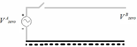
[image:3.595.309.538.83.162.2]Figure 2, The mode alpha in the transmission line.
Figure 3. The mode beta in the transmission line.
Figure 4. The mode zero in the transmission line.
The line showed in Figure 1 has the impendence and
the admittance as (10) and (11):
n nn R j L
Z (10)
n nn G j C
Y (11)
The Rn and Ln are the longitudinal parameters and Gn e
Cn are the transverse parameters of line per unit length,
considering the mode n of propagation. In the Figure 1
n AI and n
B
I are the currents at ends A and B
line, while the n
A
V and are the voltages
and these ends in the mode n. The equations for the
cur-rents in the frequency domain are given by (12) and (13):
n BV
nB AB n n
A AA n n
A Y V Y V
I
(12)
n
B BB n n
A BA n n
B Y V Y V
I (13)
The terms n
AA
Y to are evaluated as
(14) to (17):
n BB
Y
1 coth( ( )d) ZY n
C n AA
n
(14)
1 csch( ( )d)Z
Y n
C n AB
n
(15)
1 coth( ( )d)Z
Y n
C n BA
n
(16)
1 csch( ( )d)Z
Y n
C n BB
n
(17)
Equations (14) by (17), the terms n
c
Z and
n are the characteristic impendence and
propaga-tion constant in the mode n and can be written as (18)
and (19):
nnC n
Y Z
Z
(18)
n n nY Z
(19)
The n
c
Z and n
are complex numbers and
n can be written as (20).
n n n
jb a
[image:3.595.342.540.416.559.2]The real part of n
is the attenuation constant,which corresponds to the amplitude of the wave as it travels in the conductor. The imaginary part is called the
phase constant. Thus each mode of propagation n have
the characteristic impedance, attenuation constant, phase constant and propagation velocity different. As illustra-tion the simulaillustra-tion of a three-phase transmission line in to the process of energization. The physical configuration
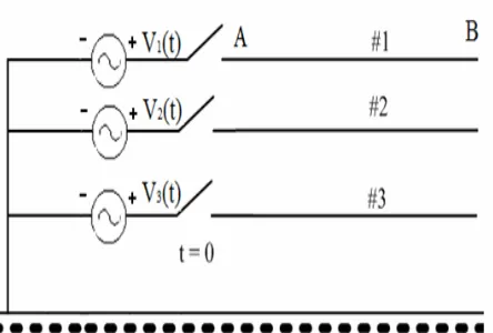
of the three-phase circuit is shown in Figure 5. The
three-phase line has the length of 100 km and frequency of 60 Hz.
5. Transient Responses due to Energization
Procedure
In the Figure 5 shows a three-phase transmission line
with the receiving open end B that will be used for the study of the model, while the phase1 is energized by a DC voltage source and the phases 2 and 3 are in short circuit in the sending end A.
The transmission line in the Figure 5 will be energized
by a DC voltage source of 20 kV. The Figures 6 to 8
show the behavior of the voltages for each propagation modes alpha, beta and zero.
The Figures 6 to 8 show the voltages in the alpha, beta, and zero modes for receiving open end of the three-phase line. It can be seen that each propagation mode behaves as a single-phase line energized by a constant voltage
Figure 5. Three-phase transmission line energized with DC source.
0 10 20 30 40 50 60
0 5 10 15 20 25 30 35
V
o
lt
ag
e m
ode
-al
pha
[
k
V
]
time [ms]
Figure 6. Voltage at the receiving end of the mode alpha.
0 10 20 30 40 50 60 70 80 -30
-20 -10 0 10 20 30
V
o
ltag
e m
o
d
e
-be
ta
[
k
V
]
time [ms]
Figure 7. Voltage at the receiving end of in the mode beta.
0 10 20 30 40 50 60 70 0
5 10 15 20 25
Vo
lt
a
g
e
m
o
d
e
-z
e
ro
[
k
V]
time [ms]
Figure 8. Voltage at the receiving end of in the mode zero.
source and each mode has a different propagation veloc-ity and different steady-state values. The values of the voltages of phases 1, 2 and 3 are obtained by linear
com-bination of the voltages modes shown in Figures 6 to 8
as (21):
qmT
clarke V
T V1,2,3 1
(21)The vector [V1,2,3] represents the voltages in phases 1,
2 and 3 and [Vqm] represents the three-phase line voltage
alpha, beta and zero modes of Figures 6 to 8. The figure
9 shows the behavior of voltage in the receiving open end B of a three-phase line, using (21).
In Figure 9 the behavior of voltage in the phase 2 and
3 are influenced by the behavior of voltage in phase 1
due to the mutual inductances of the line. The Figure 10
and 11 shows the behavior of currents in the phases 1, 2
and 3 at the receiving open end.
In the Figure 10, when the voltage in phase 1 is
posi-tive, the voltage in phases 2 and 3 become negaposi-tive, ob-eying the Faraday-Neumann’s law. When voltage in the phase 1 remains constant, the flows induced in the others phases remains constant and there is no induced voltages in the phases 2 and 3. When the phase voltage decreases, the induced voltages in the phases 2 and 3 are positive.
The Figures 10 and 11 show the same behavior obtained
in the Figure 9. Considering the three-phase
voltage source, balanced and dephased in 120o, as shown
in the Figure 12. Where Vm is the peak voltage, ω is the
angular frequency and f is the frequency. The
transmis-sion line of Figure 12 will be energized by an alternating
source of 255 V (line-neutral voltage) corresponding to a line-line voltage of 440 kV and a frequency of 60 Hz..
0 5 10 15 20 25 30 35 40 -20
-10 0 10 20 30 40
Te
nsã
o
[
k
V
]
tempo [ms]
[image:5.595.311.533.89.239.2]Phase 1 Phase 2 Phase 3
Figure 9. Voltages in the receiving end B of a three- phase transmission line.
0 20 40 60 80 100 120 140 160 180 200 -30
-20 -10 0 10 20 30
tempo [ms]
C
o
rr
e
n
te
[A
]
[image:5.595.61.285.170.322.2]Phase 1
Figure 10. The current in the sending end A of a three- phase transmission line.
0 20 40 60 80 100 120
-4 -3 -2 -1 0 1 2 3 4
tempo [ms]
C
o
rre
n
te
[
A
]
Figure 11. The current in the sending end A of a three- phase transmission line.
Figure 12. Three-phase line transmission energized with sinusoidal source.
0 5 10 15 20 25 30 35 40 45
-2 -1.5 -1 -0.5 0 0.5 1 1.5 2 2.5
time (ms)
V
o
lt
age(
pu)
[image:5.595.311.538.284.431.2]Phase 1 Phase 2 Phase 3
Figure 13. Voltages in the open end B of three-phase
trans-The voltages at the recede opening end B as shown Fi
re 13 shows that the peak voltage for a phase
1
e method of modal transformation is
is energized with a voltage source
mission line of 440 kV.
gure 13.
The Figu
reaches approximately 1.7 pu in the transient period. As the same behavior to figure 9, when the voltage in the phase 1 is a positive, in the phases 2 and 3 become nega-tives and when the voltage in phase 1 is negative, the induced voltages in the phases 2 and 3 are positives and the voltage in the system will reach the 1 pu value in steady-estate.
6. Conclusions
In this work with th
possible to obtain currents and voltages in a three-phase transmission line. Due to the difficulty of solving the second order differential equations that model the poly-phase transmission line, the system has n coupled poly-phases can be represented by n decoupled single-phase systems that are equivalent to the original system, as represented in the Figures 2 to 4.
[image:5.595.61.285.365.512.2] [image:5.595.60.284.556.708.2]D
7. Acknowledgements
by Fundação de Amparo à C in the phase 1 and the others phases are in short cir-cuit. It’s obtained the alpha, beta, and zero propagation modes, and in which each mode the velocity, attenuation and steady-state values are different, as shown in the
Figures 6 to 9. Using (21) were obtained the voltages at
receiving open end B. In the Figure 9, the peak value in
the phase 1 is approximately 2 times its steady state val-ue. At steady-state value, the voltage in the phase 1 will reach a value of DC source of 20kV and the in others phases the value steady-state will be zero because there is
no variation in mutual flow. The Figure 10 and 11 shows
the behavior of current in the phases 1, 2 and 3 of the line. When the current in phase 1 is positive, the currents in the phases 2 and 3 are negative, inducing negative volt-ages at the end B of the line. When the current in phase 1 is negative, the current in the phases 2 and 3 are positive, inducing positive voltages in the end B of the line. In the
Figure 13 the voltage in the phase 1, reaches a value of
2,0 per unit and the induced voltages in phases 2 and 3 present value of 1 pu, approximately. Thus the model of modal transformation can be used to study the transient electromagnetic transmission line phase subjected to the energization process.
This research was supported
Pesquisa do Estado de São Paulo (FAPESP).
REFERENCES
[1] S. Kurokawa, “Parâmetros Longitudinais Transversais de linhas de Transmissão Calculados A Partir das Correntes e tTensões de fase,” (Doctorate in Electrical Engineering) Faculdade de Engenharia Elétrica e de Computação,” Universidade Estadual de Campinas, Campinas, 2003. [2] C. Tavares, J. Pissolato and C. M. Portela, “Mode
Do-main Multiphase Transmission Line Model-Use in Tran-sient Studies,” IEEE Transactions on Power Delivery,
Vol. 14, No. 4, 1999, pp. 1533-1544.
doi:10.1109/61.796251
[3] P. Moreno and A. Ramirez, “Implementation of the Nu-merical Laplace Transform: A Review,” IEEE Transac-tions on Power Delivery, Vol. 23, No. 4, 2008, pp.
2599-2609.doi:0.1109/TPWRD.2008.923404
[4] S. Kurokawa and R. C. Silva, “Alternative Model of Three-phase Transmission Line Theory-based Modal Decomposition,” Revista IEEE América Latina, Vol. 10, 2012, pp. 2074-2079.