http://dx.doi.org/10.4236/am.2013.412A004
Asynchronous Approach to Memory Management in
Sparse Multifrontal Methods on Multiprocessors
Alexander Kalinkin, Konstantin Arturov ZAO Intel/AO, Novosibirsk, Russia Email: [email protected]
Received October 27,2013; revised November 27, 2013; accepted December 4, 2013
Copyright © 2013 Alexander Kalinkin, Konstantin Arturov. This is an open access article distributed under the Creative Commons Attribution License, which permits unrestricted use, distribution, and reproduction in any medium, provided the original work is properly cited. In accordance of the Creative Commons Attribution License all Copyrights © 2013 are reserved for SCIRP and the owner of the intellectual property Alexander Kalinkin, Konstantin Arturov. All Copyright © 2013 are guarded by law and by SCIRP as a guardian.
ABSTRACT
This research covers the Intel® Direct Sparse Solver for Clusters, the software that implements a direct method for
solv-ing the Ax = b equation with sparse symmetric matrix A on a cluster. This method, researched by Intel, is based on
Cholesky decomposition and could be considered as extension of functionality PARDISO from Intel® MKL. To achieve
an efficient work balance on a large number of processes, the so-called “multifrontal” approach to Cholesky decompo- sition is implemented. This software implements parallelization that is based on nodes of the dependency tree and uses MPI, as well as parallelization inside a node of the tree that uses OpenMP directives. The article provides a high-level description of the algorithm to distribute the work between both computational nodes and cores within a single node, and between different computational nodes. A series of experiments shows that this implementation causes no growth of the computational time and decreases the amount of memory needed for the computations.
Keywords: Direct Solver; Distributed Data; OpenMP and MPI
1. Introduction
The paper describes a direct method based on Cholesky decomposition for solving the equation Ax = b with sparse symmetric matrix A. The positive-definite matrix
A can be represented in terms of LLT decomposition; in
case of an indefinite matrix, the decomposition is LDLT,
where the diagonal matrix D can be amended with extra “penalty” for additional stability of the decomposition. To achieve an efficient work balance on a large number of processes, the so-called “multifrontal” approach to Cho-lesky decomposition is proposed for the original matrix.
The multifrontal approach was proposed in the papers [1,2] and successfully used in implemented algorithms [2-9]. The decomposition algorithm implementation con- sists of several stages. The initial matrix is subject to a reordering procedure [10-14] to represent it in the form of a dependency tree. The number of existing reordering algorithm is quite huge and the main aim of implementa- tion such algorithms is to achieve good width of tree (to obtain better scalability) and increase fill-in of computed L matrix. We choose metis algorithm [15] as foundation
of our project. Then the symbolic factorization takes place where the total number of nonzero elements is
computed in LLT. Then a factorization of the permuted
matrix in the LLT form takes place [4-5,7].
This work is devoted to Intel® Direct Sparse Solver for
Clusters package. This package implements paralleliza- tion based on nodes of the dependency tree using MPI as well as parallelization inside the node of tree using OpenMP directives. A variant of MPI-parallelization of Cholesky decomposition can be found in [3,7].
ferent threads in each process. This paper describes main approaches of handle elements of matrix by different processes and describes our implementation of Cholesky decomposition in one node of tree by combination of processes/threads. The proposed algorithm is based on
PARDISO functionality from Intel® MKL [16] and may
be considered as expansion of it on computers with dis- tributed memory.
The paper is organized as follows: Section 2 provides a brief description of the reordering step and describes parallel algorithms to distribute the work between both computational nodes and cores within a single node. Sec- tion 3 briefly describes the algorithm distributing a tree node between different computational nodes and pro- poses our version of handle elements of factorized matrix by different processes with using OpenMP approach on each process. Section 4 demonstrates a series of experi- ments that shows dependence working time of imple- mented algorithm of number of processes/threads and de- pendence peak of memory size needed for a process dur- ing algorithm working of number of processes.
2. Main Definitions and Algorithms
There are 2 general ways of solving system of linear equations—iterative and direct algorithms. The iterative algorithms can be more perspective but to implement they effectively one need to know information about ma- trix, like spectral analyses or differential equation which correspondent to system. Commonly this information can be achieved. On the other hand direct method could be applied for any matrix and spectral property of matrix can depend on obtained solution only. The Cholesky de- composition is the one of the direct methods.
In a general case, the algorithm of Cholesky decompo- sition can be presented in the following way:
L = A
for j = 1,size_of_matrix
{for j = 1,i
{L(i,j) = L(i,j)-L(i,k)L(k,j), k = 1,j-1 (1)
if (i==j) L(i,j) = sqrt(L(i,j)
if (i>j) L(i,j) = L(i,j)/L(j,j) }
}
Here A is a symmetric, positive-define matrix and L is the resulted lower-triangular matrix. If the initial matrix has a lot of zero elements (such kind of a matrix is called sparse), this algorithm can be rewritten in a more effi- cient way called multifrontal approach.
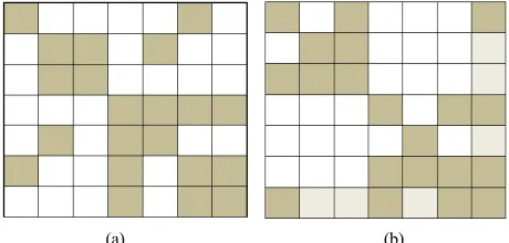
Suppose we have a sparse symmetric matrix A Figure
1(a) where each grey block is in turn a sparse sub-matrix
and each white one is a zero matrix. Using reordering algorithm procedures [15], this matrix can be reduced to
the pattern as in Figure 1(b).
(a) (b)
Figure 1. (a), (b) Non-zero patterns of original matrix and after reordering step.
A reordered matrix is essentially more convenient for computations than the initial one since Cholesky de- composition can start simultaneously from several entry
points (for the matrix from Figure 1(b), 1st, 2nd, 4th and
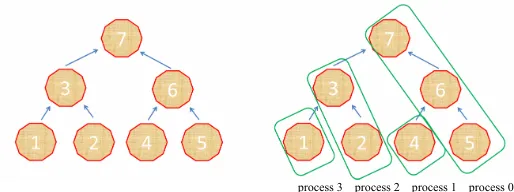
5th rows of the matrix L can be calculated independently. To be precise, a non-zero pattern of the matrix L in Cholesky decomposition is calculated at the symbolic factorization step before the main factorization step (stage). At this stage, we know the structure of the origi- nal matrix A after the reordering step and can calculate the non-zero pattern of the matrix L. At the same stage, the original matrix A stored in the sparse format is ap- pended with zeros so that its non-zero pattern matches completely that of the matrix L. Henceforth, we will not distinguish the non-zero patterns of the matrices A and L. Moreover, it should be mentioned here that elements of the matrix L in the rows 3 and 6 can be computed only after the respective elements in the rows 1, 2 and 4, 5 are computed. The elements in the 7th row can be computed at last. This allows us to construct the dependency tree [3,4,7,8]—a graph where each node corresponds to a sin- gle row of the matrix and each graph node can be com- puted only if its (nodes on which it depends) are com- puted. Deeper algorithm with pseudo code of distribution nodes of tree between processes can be finding in [13].
The dependency tree for the matrix is given in the Figure
2(a) (the number in the center of a node shows the re-
spective row number). For our example, an optimal dis- tribution of the nodes between the computational proc-
esses is given in the Figure 2(b), where the first bottom
level of the nodes belongs to the processes with the numbers 0, 1, 2, the second level belongs to 0, 2, 4, the third belongs to 0, 4, 8,···, etc.
To compute elements of LLT decomposition within a
node Z of the dependency tree, it is necessary to compute
the elements of LLT decomposition in the nodes on
which Z depends (its sub-trees). We call an update pro- cedure to bring already computed elements to the node Z (actually, this procedure takes the elements from the sub- trees of Z multiplied by themselves and subtracted from
[image:2.595.308.538.86.196.2]process 3 process 2 process 1 process 0
Figure 2. (a) Dependency tree sample; (b) Dependency tree sample distribution among processes.
non-zero pattern of Z and its sub-trees. The 4th line of the algorithm (1) completes this operation with different L(i,k) being placed into different nodes of the tree, the
last step is to calculate LLT decomposition of elements
placed into node Z. Algorithm (2) describes an imple- mentation of the above mentioned piece of the global decomposition in terms of a pseudo-code:
for current_level = 1, maximal_level
{Z = node number that will be updated by this process for nodes of the tree with level smaller than the cur- rent_level
{prepare an update of Z by multiplying elements of LLT decomposition elements lying within the current
node (2) by themselves;}
send own part of update of Z from each process to process which stores Z;
on process that stores Z compute LLTelements of Z}
Consider in details an implementation of the algo- rithms called “compute elements of Z” and “prepare an update”.
Each tree node in turn can be represented as a sub-tree or as a square symmetric matrix. To use algorithm (2),
one needs to implement LLT decomposition of each node
on a single computational process. To compute Cholesky decomposition of each node of the tree, a similar algo- rithm could be implemented on a single computational process with several threads. If the number of threads is equal to the number of nodes of the tree on the bottom
level, then LLT factors for each node from the very bot-
tom level of the tree are calculated by a single thread, on the next level each node can be calculated by 2 threads, on the next one by 4 threads, etc. However, such an algo- rithm becomes inefficient for the top nodes of the initial tree. Instead, Olaf Schenk suggested some modification of the standard algorithm of Cholesky decomposition for
sparse symmetric matrices. The standard LLT decompo-
sition for sparse symmetric matrices can be described as follows:
for row = 1, size_of_matrix
{for column = 1, row
{S = A[row, column]
for all non-zero elements in the row before the col-
umn, S = S – A[row, element]*A[element, column]; (3)
If column<row A[row, column] = S/A[column, col- umn]
else A[row, column] = S1/2;
} }
In the paper [9], the following modification of algo- rithm (3) for the computers with shared memory is pro- posed. Each computational thread sequentially selects a row or a set of k rows with similar structure (such set of
rows is called supernode) supr, for which the following
operations are performed.
for column = 1, supr
{if column is not computed - wait, otherwise do
{A[supr,*] = A[supr,*] – A[column, *]*A[column,
column];} }
A[supr, supr] = (A[supr, supr])1/2; (4) // 1/2 means Cholesky decomposition of a dense matrix that can be computed with Lapack functions
A[supr, supr + k, ···, n] = A[supr, supr + k,· ··, n] * inv
(A[supr, supr)], where inv(B) mean inverse matrix B−1;
In his paper, Olaf Schenk applies the algorithm to the entire matrix. In this paper, we apply it to the tree nodes only. Namely this provides an efficient Cholesky de- composition for a dependency tree node of the initial matrix.
The aforementioned Algorithm (4) describes an im-
plementation of the procedure в “compute elements” in
terms of the algorithm (2). The procedure “prepare an
update” differs only in a sense that each process modifies
zero columns with the structure similar to A[supr,*]
rather than A[supr,*] itself. After each process computes
its update performing simple summation, we obtain
A[supr,*] from which the computed elements of LLT
decomposition have been already deduced.
Thus, we have described the main steps of algorithm (2). It has a number of drawbacks, however. First, the number of elements of the matrix L in each process
differs significantly (for instance in the Figure 2(b), the
[image:3.595.171.428.86.182.2]stay idle expecting the next task to work on. The size of the memory necessary for each process to store elements of the matrix L differs drastically. Following the idea of algorithm 2, it can be demonstrated that all processes compute an update first, they start transferring data afterwards. This is inefficient since at this time the ma- jority of processes are idle again. To avoid the idle time
and distribute elements of LLT-factors between processes
more evenly, we propose an algorithm described in the next Section.
[image:4.595.106.238.623.713.2]3. Asynchronous Execution of Processes
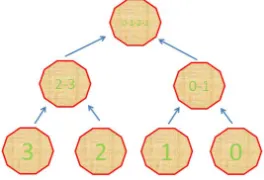
To avoid issues with uneven distribution of the elements of the matrix L, we propose a distribution method as inFigure 3 (digits in the decagons indicate the link of a
node with a given process).
Figure 3 demonstrates the same elimination tree as in Figure 2 with the elements from each node of the tree
being distributed in different manner between computa- tional processes. At each tree level but the first (bottom) one, the elements of the matrix L are stored on several processes, e.g., at the second level all supernodes are distributed between two processes, at the third one—be- tween four processes, etc. Supernodes from each node of the tree are distributed between n processes as follows: if the total number of supernodes in a certain tree node is m,
then the first group of m1 supernodes belongs to the first
process, the next group of m2 supernodes—to the second
process, etc. Here m1 + m2 + ··· + mn = m. Note that the
numbers m1, m2, ···, mn may vary that allows one to ad-
just them in order to provide better performance of the overall algorithm. Then Algorithm 2 is modified so that each process computes its part of the tree node Z. How- ever, this idea does not provide a solution to the problem of keeping processes busy during the computations. Moreover, the problem becomes even bigger since paral- lel computation of the elements of the matrix L in a sin- gle tree node is virtually impossible—almost all super- nodes in a single tree node are normally dependent on each other.
Note that each process can be executed by a modern computational node and, therefore, the node can consist of several dozens of individual computational threads.
Figure 3. Distribution of nodes among processes.
For individual processes to send/receive the data and carry out the computations, we designate one thread in each process to be a “postman”. A “postman” is a thread responsible for data transfer between the processes. Let us consider how algorithm 3 changes.
3.1. Prepare an Update
As it was stated in the Section 2, the Algorithm “prepare
an update” is a modification of the Algorithm 4. As was
mentioned before, to calculate LLT factors from node Z
of the elimination tree we need to calculate all LLT fac-
tors from its sub-trees and take them into account during
computations of LLT factors of node Z. In general case,
however, the node of the tree Z and its sub-tree are stored on different computational processes, so we cannot do it straightforwardly (node Z and its sub-tree have different non-zero pattern, for example). To resolve the issue, the following algorithm is proposed: Each computational
process i allocates matrix Zi with the same non-zero pat-
tern as the matrix corresponding to the node Z and fills it in with zero elements. Then, all elements from the sub- trees stored on the process i are taken into account in the
matrix Zi as if Zi is Z (4th line in the Algorithm 1).
Fur-ther, the computed matrices Zi are collected on the
re-quired process. Considering that we separated a post- man thread, there is no need to compute an update first, and send it later, so computations and data transfers can be interleaved.
if thread is a postman thread
{Open a recipient to get updates for supr in A_loc
{if supernode supr is computed, send it to the re-spective process;
else wait until supernode is computed; }
Else (5) {create A_loc(all elements in Z)
for supr in A_loc
{ if column on the current process
A_loc[supr,*] = A_loc[supr,*] – A[column, *] * A[column, column];
} }
the total time spent in the new algorithm is less compared to the Algorithm 4.
3.2. Compute Elements of a Tree Node
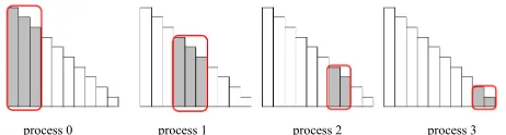
It is much more interesting to consider a more compli- cated algorithm of computing the elements of the matrix L in a single node of the tree provided that this node is distributed among several processes. Let the elements of the node Z including the elements of the dependent sub-trees (children) that are not processed yet be distrib-
uted as it is shown in the Figure 4, i.e. the first group of
supernodes belongs to the first process, and the second group—to the second one, etc. So, each computational process stores only “grey” supernodes.
It can be clearly seen that with such a distribution only the process 0 can start the computations. Thus, the first supernode can only be computed within it. However, after the supernode computation is done, it can be used by the computational threads of the process 0 for other (dependent) supernodes, second it can be sent by the postman thread to other processes, which in turn can use
it in their (dependent) supernodes (see the Figure 5,
where blue arrows indicate communications between the processes, the green ones—the update of the supernodes on each process with the supernode received from the process number 0).
With this example, it is apparent that if each process has more than 3 computational threads, some threads will simply lack a supernode to process, so making a postman out of one computational thread will have little effect on the overall efficiency if the thread count is big enough. Of course, one supernode can be processed with several threads, but this is not going to be considered in this pa- per.
4. Numerical Experiments
All numerical experiments in this paper were carried on
[image:5.595.58.289.553.615.2]process 0 process 1 process 2 process 3
Figure 4. Supernode distribution among the processes.
process 0 process 1 process 2 process 3
Figure 5. Computational flow.
the Infiniband*-linked cluster consisting of 16 computa-
tional nodes; each node contains two Intel® Xeon®
X5670 processors (12 cores in total) with 48Gb of RAM per node. The variable number of the computational
threads within a node is created, i.e. only part of totally
available threads is working within the nodes in the most cases.
4.1. Scaling of Computational Time
For this experiment, we selected either 7-diagonal matrix resulted from the approximation of a Helmholtz equation on a uniform grid with a positive coefficient (specific Helmholtz coefficient value is not crucial here since it has no effect on the matrix structure and only the accu- racy of the solution obtained depends on it), or the matrix generated from the oil-filtration problem. The number of degrees of freedom (NDOF) for the first matrix is about 398 K elements, for the second one is about 1.7 M, and the number of nonzero elements (NNZ) in each matrix is 15.7 M and 12 M, respectively.
The exact solution corresponds to unit vector – array with all elements equal to 1. Need to underline that per- formance of whole algorithm doesn’t depend on choos- ing rhs.
Figures 6-7 show acceleration of Intel®Direct Sparse
Solver for Clusters code on a different number of proc- esses compared to the same program launched on 1 MPI process with 2 OpenMP threads on different matrices. The colored lines correspond to a different number of OpenMP threads used in the code. It can be seen from the Figures that the execution time reduces in all cases with the increase of the number of threads and processes. It can be readily seen that sometimes even super-linear acceleration takes place depending on the number of OpenMP threads that can be easily explained from the nature of the algorithm one thread is used to send& re- ceive data and rather often it falls out of the computa- tions. For example, in the case of 2 threads, one thread is the postman and the other is the computational one, in
0
Number of MPI precesses (1 per HW node) NDOF = 398 K, NNZ = 15.7 M
Time scalability (higher is faster)
Speed-up vs
.M
PI
= 8,
OM
P =
2 conf
igur
ati
on
OMP=2 OMP=4 OMP=8 OMP=12
8 16 4
2 1
5 10 15 20 25
0
Number of MPI precesses (1 per HW node) NDOF = 1.7 M, NNZ = 12 M Time scalability (higher is faster)
Sp
eed-up vs
.M
PI
= 8,
O
M
P = 2 conf
igur
ati
on
OMP=2 OMP=4 OMP=8 OMP=12
8 16 4
2 1
[image:6.595.60.287.83.244.2]5 10 15 20 25 30 35 40
Figure 7. Intel ® direct sparse solver for clusters scalability of time.
the case of 4 threads, one thread is the postman and 3 others are computational ones.
Based on the Figures, it can be concluded that it is rec- ommended to exploit the computational threads on the node to the maximum and it is not recommended to have several computational processes per one node. From the
Figure 6, it is apparent that the acceleration of the com-
bination 2 MPI x 8 OpenMP is larger than 4 MPI x 4 OpenMP, that in turn, is larger than 8 MPI x 2 OpenMP. This perfectly matches the architecture features imposed by the modern computer systems, namely, the growing number of cores (threads) per computational node. Need to underline that in case of 1 MPI process SMP Pardiso functionality from Intel MKL 10.3.5 [16] have been used. So we can conclude that MPI version of proposed algo- rithm works better than corresponded SMP version on one node.
4.2. Memory Scaling Per Node
We use the same matrices as before for the testing pur-
poses. In the Figures 8-9, the maximal memory size
needed for a computational node depending on the num- ber of nodes is presented.
Memory size that Intel® Direct Sparse Solver for
Clusters needs for every computational node barely de- pends on the number of computational threads on it. Therefore, we present the data for the number of threads equal to 12 only. It is apparent that the memory size that every process needs demonstrates inverse dependence on the number of processes (for the second matrix, the memory required decreased 5 times for 16 processes vs. 1 process). If the computational cluster has insufficient memory per node, it is still possible to solve the system
of linear equations using Intel® Direct Sparse Solver for
Clusters package increasing the number of nodes in the cluster. An example of this will be shown in the fol- lowing paragraph.
8 16
0
Number of MPI precesses (1 per HW node) NDOF = 1.7 M, NNZ = 12 M Absolute memory per node scalability
M
ax mem
or
y per
node,
Gb
4 2
1
(Lower is better)
1 2 3 4 5 6 7
Figure 8. Intel® direct sparse solver for clusters memory scalability.
8 16
0 2 4 6 8 10 12 14 16 18
Number of MPI precesses (1 per HW node) NDOF = 1.7 M, NNZ = 12 M Absolute memory per node scalability
M
ax mem
or
y per
node,
Gb
4 2
1
[image:6.595.310.537.83.228.2](Lower is better)
Figure 9. Intel® direct sparse solver for clusters memory scalability.
4.3. Solving a Huge System of Linear Equations
In this paragraph, we chose a matrix of size 5.8 M with more than half a billion non-zero elements for the ex-
periment. Thanks to Intel® Direct Sparse Solver for Clus-
ters memory scaling, we can solve this system on 8+ MPI processes. Note that almost 40 GB of memory is required per process in case of 8 MPI processes. For 16 processes,
29 GB of memory is only required (see Figure 10-11).
In Figures 10-11, the comparison of computational
time with the configuration 8 MPI x 2 OpenMP is pre- sented. It is clear that even for such a big matrix size and
big number of MPI processes, Intel® Direct Sparse
Solver for Clusters shows good scalability both in terms of OpenMP threads and MPI processes.
5. Conclusion
Within the frameworks of multifrontal approach, we proposed an efficient algorithm implementing all stages of Cholesky decomposition inside the node of the de- pendency tree for all processes on a distributed memory
machine. This approach is implemented in Intel® Direct
[image:6.595.309.537.265.419.2][2] J. W. H. Liu, “The Multifronal Method for Sparse Matrix Solution: Theory and Practice,” Siam Review, Vol. 34, No. 1, 1992, pp. 82-109. http://dx.doi.org/10.1137/1034004
8 16
0
Number of MPI precesses (1 per HW node) NDOF = 5.8 M, NNZ = 500 M Scalability of (computational) time
Speed-up vs
.M
PI
= 8,
OM
P = 2 conf
ig
ur
ati
on
1 2 3 4 5 6 7 8
OMP=2 OMP=4 OMP=8 OMP=12
[3] P. R. Amestoy, I. S. Duff and C. Vomel, “Task Schedul- ing in an Asynchronous Distributed Memory Multifrontal Solver,” SIAM Journal on Matrix Analysis and Applica- tions, Vol. 26, No. 2, 2005, pp. 544-565.
http://dx.doi.org/10.1137/S0895479802419877
[4] P. R. Amestoy, I. S. Duff, S. Pralet and C. Voemel, “Adapting a Parallel Sparse Direct Solver to SMP Archi- tectures,” Parallel Computing, Vol. 29, No. 11-12, 2003, pp. 1645-1668.
[image:7.595.58.293.85.226.2]http://dx.doi.org/10.1016/j.parco.2003.05.010
Figure 10. Intel® direct sparse solver for clusters time scal-ability, a huge system.
[5] P. R. Amestoy, A. Guermouche, J.-Y. L’Excellent and S. Pralet, “Hybrid Scheduling for the Parallel Solution of Linear Systems”, Parallel Computing, Vol. 32, No. 2, 2006, pp. 136-156.
http://dx.doi.org/10.1177/109434209300700105
8 16
0 5 10 15 20 25 30 35 40 45
Number of MPI precesses (1 per HW node) NDOF = 5.8 M, NNZ = 500 M Scalability of the total memory needed per node
Ma
x
m
em
or
y per
n
od
e,
G
b [6] P. R. Amestoy and I. S. Duff, “Memory Management
Issues in Sparse Multifrontal Methods on Multiproces- sors,” The International Journal of Supercomputer Ap- plications, Vol. 7, 1993, pp. 64-82.
[7] P. R. Amestoy, I. S. Duff, J.-Y. L’Excellent and J. Koster, “A Fully Asynchronous Multifrontal Solver Using Dis- tributed Dynamic Scheduling,” SIAM Journal on Matrix Analysis and Applications, Vol. 23, No. 1, 2001, pp. 15- 41. http://dx.doi.org/10.1137/S0895479899358194 [8] M. Bollhofer and O. Schenk, “Combinatorial Aspects in
Sparse Direct Solvers,” GAMM Mitteilungen, Vol. 29, 2006, pp. 342-367.
Figure 11. Intel® direct sparse solver for clusters memory
scalability, a huge system. [9] O. Schenk and K. Gartner, “On Fast Factorization Pivot- ing Methods for Sparse Symmetric Indefinite Systems,” Technical Report, Department of Computer Science, University of Basel, 2004.
experiments show good scaling in computational time— proportional to the number of computational nodes used and the number of threads within them. Such scaling can be achieved only by scaling all substeps of Cholesky decomposition. The main issue on this algorithm, fac- torization of node of tree by several processors, has been implemented via approach presented in this paper. Be- sides, this algorithm reduces the requirement for the memory size used by the algorithm on a single node when the number of processes grows. The experiments made the confirmation of it.
[10] G. Karypis and V. Kumar, “Parallel multilevel graph partitioning,” Processing of 10th International Parallel Symposium, 1996, pp. 314-319.
[11] G. Karypis and V. Kumar, “A Parallel Algorithm for Multilevel Graph Partitioning and Sparse Matrix Order- ing,” Journal of Parallel and Distributed Computing, Vol. 48, 1998, pp. 71-85.
http://dx.doi.org/10.1006/jpdc.1997.1403
[12] K. Schloegel, G. Karypis and V. Kumar, “Parallel Multi- level Algorithms for Multi-Constraint Graph Partitioning” Euro-Par 2000 Parallel Processing, 2000, pp. 296-310
6. Acknowledgements
[13] A. Pothen and C. Sun, “A Mapping Algorithm for Paral-lel Sparse Cholesky Factorization,” SIAM: SIAM Journal on Scientific Computing, Vol. 14, No. 5, 1993, pp. 1253- 1257. http://dx.doi.org/10.1137/0914074
The authors would like to thank Sergey Gololobov for providing feedback that improved both style and content
of the paper. [14] G. Karypis and V. Kumar, “Parallel Multilevel Graph
Partitioning,” Proceedings of the 10th International Par-allel Processing Symposium, 1996, pp. 314-319.
REFERENCES
[15] Metis, http://glaros.dtc.umn.edu/gkhome/views/metis[1] I. S. Duff and J. K. Reid, “The Multifrontal Solution of Indefinite Sparse Symmetric Linear,” ACM Transactions on Mathematical Software, Vol. 9, No. 3, 1983, pp. 302- 325. http://dx.doi.org/10.1145/356044.356047
[16] MKL, Intel® Math Kernel Library
[image:7.595.58.288.262.409.2]