Computing Approximation GCD of Several Polynomials by Structured Total Least Norm

(1)

http://dx.doi.org/10.4236/alamt.2013.34008

Computing Approximation GCD of Several Polynomials

by Structured Total Least Norm

*

Xuefeng Duan1, Xinjun Zhang1, Qingwen Wang2 1

College of Mathematics and Computational Science, Guilin University of Electronic Technology, Guilin, China 2

Department of Mathematics, Shanghai University, Shanghai, China Email: [email protected]

Received September 28, 2013; revised October 30, 2013; accepted November 8,2013

Copyright © 2013 Xuefeng Duan et al. This is an open access article distributed under the Creative Commons Attribution License, which permits unrestricted use, distribution, and reproduction in any medium, provided the original work is properly cited.

ABSTRACT

The task of determining the greatest common divisors (GCD) for several polynomials which arises in image compres- sion, computer algebra and speech encoding can be formulated as a low rank approximation problem with Sylvester matrix. This paper demonstrates a method based on structured total least norm (STLN) algorithm for matrices with Sylvester structure. We demonstrate the algorithm to compute an approximate GCD. Both the theoretical analysis and the computational results show that the method is feasible.

Keywords: Sylvester Matrix; Approximate Greatest Common Divisor; Low Rank Approximation; Structured Total Least Norm; Numerical Method

1. Introduction

Let deg



 

In this paper, we consider the following problem. Let

 

1 ,

f x f₂

 

x , , f_t

 

x C x

 

\ 0

 

, namely



f x be the degree of f x

 

and C x

 

be the set of univariate polynomials. A₂ stands for the spectral norm of the matrix A. _Cn and _Cm n

are the vector spaces of complex n vectors and m n

matrices, respectively. Transpose matrices and vectors are denoted by _AT

and . denotes the

greatest common divisor for the polynomials

T

u GCD f



,g



f and

g. We use rank



A



to stand for the rank of matrix

A.

 

1 n n1 ,

1 n n

1 0

f x a x a _x    a xa

 

1

( 1) 1 0, 2, ,

p p

i ip i p i i .

f x b x b _ x    b xb i  t

Problem 1.1. Set k be a positive integer with





min ,

k n p . We wish to compute f1

 

x , f2

 

x , ,

 ft

 

x C x

 

\ 0

 

, such that

 



1





 



deg f x n, deg f_i x  p, 2 i t,

 

   

 







1 1 2 2



deg GCD f x  f x ,f x  f x ,,ft x  ft x k,

and

 

2

 

2

 

1 ₂ 2 ₂ t

2

f x f x f x

     

is minimized.

The problem of computing approximate GCD of several polynomials is widely applied in speech encoding and filter design [1], computer algebra [2] and signal pro- cessing [3] and has been studied in [4-7] in recent years.

Several methods to the problem have been presented. The generally-used computational method is based on the truncated singular decomposition(TSVD) [8] which may not be appropriate when a matrix has a special structure since they do not preserve the special structure (for example, Sylvester matrix). Another common method based on QR decomposition [9,10] may suffer from loss of accuracy when it is applied to ill-conditioned problems and the algorithm derived in [11] can produce a more accurate result for ill-conditioned problems. Cadzow algorithm [12] is also a popular method to solve this problem which has been rediscovered in the literature [13]. *_{The author is supported by a grant from National Natural Science}

(2)

Somehow it only finds a structured low rank matrix that is nearby a given target matrix but certainly is not the closet even in the local sense. Another method is based on alternating projection algorithm [14]. Although the algorithm can be applied to any low rank and any linear structure, the speed may be very slow. Some other methods have been proposed such as the ERES method [15], STLS method [16] and the matrix pencil method [17]. An approach to be described is called Structured Total Least Norm (STLN) which has been described for Han- kel structure low rank approximation [18,19] and Sylves- ter structure low rank approximation with two polynomials [20]. STLN is a problem formulation for obtaining an approximate solution



AE X



 B H to an overdetermined linear system

AX B preserving the given structure in A or



A B



.

In this paper, we apply the algorithm to compute the structured preserving rank reduction of Sylvester matrix. We introduce some notations and discuss the relationship

between the GCD problems and low rank approximation of Sylvester matrices in Section 2. Based on STLN method, we describe the algorithm to solve Problem 1.1 in Section 3. In Section 4, we use some examples to illustrate the method is feasible.

2. Main Results

First of all, we shall prove that Problem 1.1 always has a solution.

Theorem 2.1. Suppose that f1, f2, , ft ,

 

1

deg f , deg

 

f₂ , , deg



f_t



and are defined as those in Problem 1.1. There exist

k

1

ˆ

f , fˆiC x

 

with deg

 

fˆ1 n, deg

 

fˆi  p and







_fˆ



_

1 2 t

ˆ ˆ_, _, _,

f f 

deg GCD k su ch th at for all f1,

 

i

f C x w i t h deg

 

f1 n , deg

 

fi  p a n d







1 2



deg GCD f,f ,,f_t k, 2 i t. We have

2 2 2 2 2

1 1 2 2 1 1 ₂ 2 2 ₂

2 2 2

ˆ ˆ ˆ _.

t t t t

2

f f  f  f   f  f  f f  f  f   f  f

Proof. Let hC x

 

be monic with deg

 

h k and set uiC

 

x with deg

 

ui deg



fi



k

h

. For the real and imaginary parts of the coefficients of and of

. We are considered with the continuous ob- jective function

, i

u



1 i t







2 2

1 2 1 1₂ 2 2 ₂

2 2 , , , ,

. t

t t

F h u u u u h f u h f

u h f

   

  



We will prove that the function has a value on a closed and bounded set of its real argument vector which is smaller than elsewhere. Consider 1

n n

f a x and

p i ip

f b x with a GCD of degree k for 2 i t. Clearly, any h and ui with





2 2 2

1 2 1 1₂ 2 2 ₂ ₂

, , , , t > t t

F h u u u f  f  f  f   f  f

can be discarded. So from above,we know that the

coefficients of 1 2 can be bounded

and so can the coefficients of 1 2 t by

any polynomials factor coefficient bound. Thus the ,

u h u h, ,

h

t

u h

, u, u , , u

function’s domain F h u u



, 1, 2,,ut



0

is restricted to a sufficiently large ball. It remains to exclude

1 2 t

u u u  as the minimal solution. We have





2 2 2

1 2 2 2 2

2 2

1 1 ₂ 2 2 ₂

, 0, 0, , 0 _t

t t

F h f f f

2 2

f f f f f f

   

      

 

 .

In conclusion, the theorem is true.

Now we begin to solve Problem 1.1, we first define a





p n p matrix associated with f₁

 

x as follows

1 2 1 0

1 1 0

1

1 1

0 0

0

, 0

0 0

n n n n n

n n

a a a a a

a a a a

S

a a a a

  

 0

 

 



 

 

 

  

    

  

and an n 



n p



matrix associated with f x_i

 

,

2, 3, ,

i  t as

















1 0

1 2 0

0 1 0

,

0

0 0 1

ip i i i i

ip i i i

i

ip i i i

b b p b p b b

b b p b b

S

b b p b b

 

 

 _ 

 



 

 _ 

 

 

  

     

     

  

0

0 



(3)

    

T 1

1 2

.

p n t n p

t

S S

S C

S

   

     

 

     



Deleting the last k1 rows of S and the last k1 columns of coefficients of f1,f2,,ft separately is

, We get the -th Sylvester matrix

S k

n p k 1  t1n p tk t Sk C

  

     

   

2

1 2 1 1

2

0 1 10 2 1 0 1

0 20

0

.

n p tp

n p t p

n p

k

n p t t

t

a b b

a b

S

a a b b b b

a b

  

0

tp p

b

 

 



 

 



   

      



      



It is well-known that deg



GCD f



1ft



k if and

only if has rank deficiency at least 1. We

have



1

k

S f f_t



 

1

2 2

1 1 ₂ 2 2 ₂

deg

2 2

1 1 ₂ 2 2 ₂

dimNullspace 1

min

. min

t

k

t t GCD f f k

t t S

f f f f f f 2

2

f f f f f f



     

     



 

(2.1) where Sk is the k-th Sylvester matrix generated by

1,

f f₂, , ft.

From above, we know that (2.1) can be transformed to the low rank approximation of a Sylvester matrix.

If we use STLN [16] to solve the following overdetermined system

,

k k

A X b

for Sk 



bk Ak



, where k is the first column of k

and k

b S

A are the remainder columns of k, then we get a

minimal perturbation

S



hk Ek



of Sylvester structure sa-

tisfying

.

k k k k

b  h A E

So the solution with Sylvester structure is





k k k k k

S  h b E A and dimNullspace

 

Sk > 1. We will give the following example and theorem to explain why we choose the first column to form the overdetermined system.

Example 2.1. Suppose three polynomials are given

 

2

1 1,

f x x 

 

2

2 2,

f x x  x

 

2

3 2 3

f x x  x .

The matrix S is the Sylvester matrix generated by

 

1 ,

f x f₂

 

x and f3

 

x

1 0 1 0 1 0

0 1 1 1 2 1

1 0 2 1 3 2

0 1 0 2 0 3

S

 

 



   

 _ _ _ 

 

The matrix S is partitioned as S b Aˆ1 ˆ1 or 1 1

S A b_ , where 1 is the first column of , whereas

ˆ

b S

1

b is the last column of S. The overdetermined system

1 ˆ1 ˆ

A X b

has a solution X 



1 1 1 1 1



T, while the system

1 1

A X b

has no solution.

Theorem 2.2. Suppose that f1, f2, , ft ,

 

1

deg f , deg

 

f₂ , , deg



f_t



and are defined as those in Problem 1.1 and is the -th Sylvester matrix of 1

k k

k

S

,

f f2, , ft . Then the following

statements are equivalent. 1) dimNullspace

 

S_k 1;

2) A Xk bk has a solution, where bk is the first

column of Sk and Ak are the remainder columns of

.

k

S

Proof.  Suppose A Xk bk has a nonzero

solution, then kRange

 

. b

k

b A Since bk s the first co-

lumn of Sk, viously, the dimension of the rank de-

ficiency of

i o





k

S k k least 1.

Suppose the rank deficiency of

b A

 is at

 S_k 



b_k A_k



is

at least 1 and D x

 

GCD f



1,f2,,ft



,

 

*

1 1 ,

f  f D x f2* f2 D x

 

, ,

 

*

t t

f  f D x

1

, p k , ,1

x    x

  

.

Multiplying the vector _ _ to

the matrix , then we obtain

n p

V  x k n k

S

1

1, 1, , 1, 2, , 2, , , , .

p k p k n k n k

k t t

(4)

Next we will prove that A Xk bk has a solution. If

we multiply the vector V to two sides of the equation

k k

A X b , it turns out to be

1

1 1 2 2

1

, , , , , , , , ,

.

p k n k n k t t p k

x f f x f f x f f x f

   



 



    X

(2.3)

The solution X of equation (2.3) is equal to the coefficients of polynomials u1, u2, , ut such that

1 1 1 2 2 .

p k

t t

x  f u f u f   u f

We can get deg



D x

 



k and deg

 

f1*  n k,

 

*

deg fi  p ,

dimNullspace S

k



2 i t



 

k 1

from

. Dividing xp k by 2* t

*

f   f

m

, we obtain a quotient q and a remainder satisfy



* *



2 .

p k

t

x  q f   f m

where deg

 

q deg



D x

 



k, deg

 

m   p k 1 . Now we can get that

* *

1 , 2 1, , t

u  p u mf  u mf1. are solutions of Equation (2.3), since

 

1



 



deg u deg D x k,

 





 

* 1

deg deg deg

deg deg ,

i

u q f

D x k f n k

 

    

and



* *



1 1 2 2 2 .

p k

t t t

u f u f   u f  fq f   f  fp fx 

Next, we will illustrate for any given Sylvester matrix,

as long as all the elements are allowed to be perturbed, we can always find k -Sylvester structure matrices



hk Ek



satisfy k k , where k

is the first column of and



Range

b h A E

k



k k k

S

b A are the remainder column of k.

Theorem 2.3. Given the positive integer , there

exists a Sylvester matrix with rank

deficiency k.

S

, ,

n p t

n

n pp t1

SC    

Proof. We can always find polynomials

 

1, 2, , t

f f  f C x with deg

 

f1 n,

 

deg fi  p, 2 i t and deg



GCD



f1,f2,,ft



k 1, 2, , t

. Hence S is the Sylvester matrix of f f  f and its rank deficiency is k.

Corollary 2.1. Given the positive integer , and -th Sylvester matrix

, ,

n p t k Sk 



A bk k



 , where

n p k 1pt1ntk t Ak C

     



k

 

k

b C

, , it is always

possible to find a -th Sylvester structure perturbation n p k   1 1



hk Ek



such that bk  hk Range



AkEk



.

3. STLN for Overdetermined System with

Sylvester Structure

In this section, we will use STLN method to solve the overdetermined system

,

k k

A X b

According to theorem 2.3 and corollary 2.1, we can always find Sylvester structure



hk Ek



with





Range

k k k k

h  b A E . Next we will use STLN me-

thod to find the minimum solution.

First, we define the Sylvester structure preserving perturbation [hk Ek] of Sk





 

   

 

1 2 2

2 3 2 1

1 2 2

1 2 2 3 1 2

1 2 1

n n t p t

k k

n n p n n t p t n t p t

n n p n t p t

z z z

h E

z z z z z z

z z z

   

    

   

          

     

 

 

  

 

 



   

      



      



1

can be represented by a vector

 

T 1, 2, , n t 1p t

Z  z z  z _{ } _ _ .

We can define a matrix Pk such that hk P Zk .

 1  1 

1 0

,

0 0

n p k n t p t n

k

I

P _  _C       

 

where In1 is a



n  1

 

n 1



identity matrix.

We will solve the equality-constrained least squares problem

2 2 ,

, subject to 0. min

Z X

Z r (3.1)

where the structured residual r is



,



_k _k



_k _k



.

rr Z X b h  A E X

By using the penalty method, the formulation (3.1) can be transformed into





2

,

2

,

, 1

min Z X

wr Z X w

(5)

where is a large penalty value. Let

w

Z

 and X stand for a small change in Z X , res

,

Z



and p be the correspondi

rder approximat ectively and

i

k

change in E . Then the first o

E

 ng

e to

k



Z X X



s





r





k k

r Z Z X X b P Z Z

















,

.

k k k

k k k k k k k k

A E E X X b P Z A E X P Z

A E X E X

    

     

    

Introducing a matrix of Sylvester structure and



(3.2) can be approximated by

k

Y

 

 

T 1, 2, , p t 1n tk t 1

X x x  x _{ } _{  }









 

, ₁

min

0

X Z _n _t _{p t}

2 k k k k

w Y P w A E Z wr I

  __ _{ } _ __ X Z

      

 _   

    (3.3)

where satisfies that

(3.4)

e following, we presen btain the

matrix . Suppose

n p k 1n t1p t

k

Y C       

.

Y Zk E Xk

In th t a method to o

k

Y f₁, f₂, , f_t, E, Z and

X are d fined as abo

1_

to th

e ve. Multiplying the vector

1

, n p k n p k

V  x  x   x 

e two sides of equation (3.4), it becomes

, ,, ,

. k k

VY ZVE X

Let Xˆ 0 X

 

_{ }, we obtain

 





ˆ 1 1ˆ ˆ ˆ2 2 ˆ ˆ , kX V hk k  ˆu g u  g u

VE E X g  _t _t (3.5)

where gˆ1

ed

is the polynomial with degree which is generat by the subvector of

n

Z:



z1 z2  zn1



,

2 ˆ

g is the polynomial with degree which is rated by the subvector of

p

gene Z:

2 3 2 ,

n n n p

z_ z_ z _{ }

      ˆ_t g by the

is the polynomial with degree wh h is generated subvector of

p ic

Z:

l w egree which is ge-

ed by the subvector of

 2  2 1  1 ,

n t p t n t p t n t p t

z_{ } _ z _{ } _{ } z_{ } _

 

  

ˆ

u1 is the polynomia ith d nerat

1

p k X:

de which is

generated by the subvector of

1

0 x xp k ,

 

  

2 ˆ

u is the polynomial with gree n k

X:

1 2 2

p k p k n p k

x   x   x  1 ,

      ˆ_t u rate

is the polynomial with de wh h is gene-

d by the subvector of

gree n k ic

X:

 2  1 1  2  1  1 1 ,

p t n t k t p t n t k t p t n tk t

x _{ } _{ } _{ } x _{ } _{ } _ x _{ } _{  }

 

 

Here we will present simp



a le example to illustrate how to find

Exampl 1. Suppose ,

k

Y .

e 3. k1 X 



x x1, 2,,x7



and

 

3 2

1 3 2 1 0,

f x a x a x a xa

 

2

2 22

f x b x b21x b 20,

 

2

3 3 31 .

f x b x₂ b x b

32 31 30 1 0 0 b b 30  22 3

3 21 22 32 2

2 20 21 22 31 32 1 1

1 20 2 30 31 0

0 2 30

0 0 0 0 0

0 0

, ,

0 0

0 0 0 0

b b a

a b b b a

A a b b b b b b a

a b b b b a

a b b

                             _{ }   then 6 7 . 2 5

1 3 2 6 5

1 1 4 3 2 7 6 5

3 7

1 4

0 0 0 0 0 0 0

0 0 0 0 0

0 0 0

0 0 0 0 0

0 0 0 0 0 0

x x

x x x x x

Y x x x x x x

1 4

0

x

x x x x x

x x x

                

4. Approximate GCD Algorithm and

Experiments

Problem The following algorithm is designed to solve

1.1.

Algorithm 4.1.

Input-A Sylvester matrix S generated by f1, f2,

,

 ft, respectively, an integer k and a tolerance

tol.

Output-Polynomials f₁, f₂, , ft and the -

ea distance

Eu clid n f1 f1₂2 f2 f2 2₂  ftft 2₂ is

to

-th Sylvester matrix as the ab

rst column of and the

as a minimum.

1) Form the k ove

section, set the f re-

mainder column

k

S

as b

i s of

k

S _k

k k

S A . Let E_k 0, h_k 0. 2) Calculate X from min A X_k b_k ₂ and

k k

rb A X . Compute Pk and Yk as th above sec-

tion.

e

3) Repeat

(1)









 

, X Z

  __ ₁ __

2 . min

0 k n t p t

w

I _{ } _ X  Z

 _{ }_   

   

k k k

w Y P A E Z wr

(6)

, ,

X X X Z   Z Z

(2) Let

(3) Form the matrix Ek and hk from Z, and from

k

Y X. Let A_k A_k E_k,

A

 

 

,

h r b

k k

b b  _k _k _kX until X ₂ tol and

2

Z tol

4) tput t 

Ou he polynomials f1, f2, , ft con-

structed from



_k A_k



.

nce

b

Given a tolera , we can use the Al m 4.1 to

co f

gorith mpute an approximate GCD o f1,f2, , t

p using Algorith

f

ith m 4.1

 . The me-

thod begin w kmin

 

n,

to compute the minimum perturbation 2

2 i i i

N



f  f

with dimNullspace

 

S 1. If N <, then we can com- . Otherwise, pute the approximate GCD form matrix

we reduce k by one and repeat the Alg

k

S

orithm 4.1.

mple 4.1. We wish t d the m

Exa o fin inimal polynomial

perturbations f and g of 2

6 5,

f x  x 2

6.3

gx  x5.72,

satisfy that the polynomials  f f and  g g

ount.

have a common root. We take two

Case 1: The leading coefficients can e perturbed. Let

iteratio get the

cases into acc b

1

k and _tol_₁₀3

, after 3 ns, we poly-

nomials f and g

2

0.9850 6.0029 4.9994,

f  x  x

2

1.0 5

g 1 0x 6.2971x5.7206,

with a minimum distance

2 2

2

2 0.0004663.

N f f  gg 

nts can be perturbed. Let and after 3 iterations, we have the po-

ials

Case 2: The leading coefficie 1

k

lynom

3 10

tol  ,

f and g: 2

6.0750 4.9853,

f x  x

2

6.222 5.7353,

g x  x

2 2

2

2 0.01213604583.

N f f  gg 

and

,

after 8 iterations, we have the polynomia

Example 4.2. Let k1, tol103

3 2

1 1.98 5 5 2.96,

f  x  x  x

2

2 1.9 1,

f  9x 1.01 3.0

2

3 2 4.99 2.99

f  x  x

ls

3 2

1 1.9800 5.0000 5.0000 2.9600,

f  x  x  x

2

2 1.9963 1.0100 3.009

f  x  x

2

3 2.0071 4.9900 2.9902,

f  x  x

2 2 2 ₅

1 1₂ 2 2 ₂ 3 3 ₂ 9.0763 10 ,

N  f  f  f  f  f  f   

and the CPU time

 

0.974920

t s

Example 4.3. Let k1., tol103 and

4 3 2

1 1.85 2 2.69 1.42 ,

f  x  x  x  x

3 2

2.9 x 1.18x

 

2 1.47 4 2.36,

f  x 

3 2

3 0.52 4.01 5.94 ,

f  x  x  x

after 11 iterations, we have the polynomial

3 2

4 0.52 0.13 1.05 2.58.

f  x  x  x

s

4 3 2

1 1.85 2 2.69 1.42 ,

f  x  x  x  x

9,

3 2

2 1.47 2.94 1.18 2.36

f  x  x  x ,

3 2

3 0.5242 4.01 5.9405 ,

f  x  x  x

3 2

4 0.52 0.134 1.05 2.58.

f  x  x   x

2 2 2 2

1 1 ₂ 2 2 ₂ 3 3 ₂ 4 4 ₂

5 3.4387 10 ,

 

N f f  f  f  f  f  f f

and the CPU time

 

0.642582 .

t s

Example 4.4. Let k2, 3 10

tol  and

4 3 2

1 0.144 0.761 1.316 0.74 ,

f  x  x  x  x

after 1 iteration, we have the polynomials 3

2 0.393 12 2.56

f  x __2.2 _x2__4.132x

3 2

3 0.182 0.358 0.752 1.48,

f  x  x  x

3 2

4 0.173 0.544 0.01 0.592.

f  x  x  x

4 3 2

1 0.144 0.761 1.316 0.74 ,

f  x  x  x  x

3 2

2 0.393 2.212 4.132

f  x  x  x2.56,

3 2

3 0.182 0.3548 0.752 1.48,

f  x  x  x

3 2

4 0.173 0.4701 0.01 0.6257

f  x  x  x .

2 2 2 2

1 1 ₂ 2 2 ₂ 3 3 ₂ 4 f4 ₂

N f f  f  f  f  f  f 

and the CPU time 0.0066,

(7)

Example 4.5. Let , and

after 1 iteration, we have the polynomials

4

 

0.001335 .

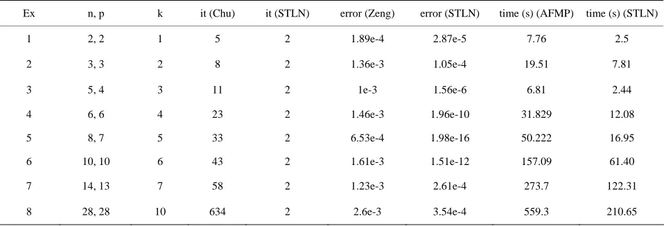
t s In Table 1, we present the performance of Algorithm 4.1 and compare the accuracy of the new fast algorithm with the algorithms in [9,21]. Denote be the total degree of polynomials

n

1

f and be the total degree of polynomials

p

, 2

i

f  i t. It (Chu) stands for the number of iterations by the method in [14] whereas it (STLN) denotes the number of iterations by Algorithm 4.1. Denoted by error(Zeng) and error (STLN) are the

2

k tol103

6 5 4

3 2

4 2.56 2.56

0.62 1.03 3.32 5.8,

x x x

 

   

1 0.6

f 

5 4

2 1.85 5.7 2.84,

f  x  x 1.31x33.96x2

5 4 3 2

3 0.44 3.23 7.64 4.7 4.72 4.72,

f  x  x  x  x  x

perturbations 2

2 i i i f f



computed by the method in

5 4 3 2

4 1.23 4.92 2.65 9.645 11.12 2.04,

f  x  x  x  x  x

[21] and Algorithm 4.1, respectively. The last two columns denote the CPU time in seconds costed by AFMP algorithm and our algorithm, respectively.

5 4 3 2

5 1.31 5.76 8.49 5.47 0.48 5.16.

f  x  x  x  x  x

As shown in the above table, we show that our method based on STLN algorithm converges quickly to the minimal approximate solutions, needing no more than 2 iterations whereas the method in [14] requires more iteration steps. We also note that our algorithm still converges very quickly when the degrees of polynomials become large while the algorithm in [14] needs more iteration steps. Besides, our algorithm needs less CPU time than the AFMP algorithm. So the convergence speed of our method is faster. From the errors, we demonstrate that our method has smaller magnitudes compared with the method in [21]. So our algorithm can generate much more accurate solutions.

6 5

1

3 2

0.6401 2.56 2.5603

0.62 1.03 3.32 5.8,

f x x x

x x x

  

   

5 4 3

2 1.85099 5.7 1.3102 3.9

f  x  x  x  6x22.84,

5 4

3

2

0.4389 3.23 7.64

4.7003 4.72 4.72, 3

f x x

x x

  

  

x

5 4 3 2

4 1.23 4.92 2.65 9.645 11.12 2.04,

f  x  x  x  x  x

5 4

5

2

1.307 5.76 8.4902

5.47 0.48 5.16. 3

f x x

x x

  

  

x

_{5. Conclusion}

2 2

1 1₂ 2 2 ₂ 3 3

2

2 2

5 5 ₂

1.1460 10 ,

N f f f f f f f f f f

     

   

 

and the CPU time

Examples 4.1, 4.2, 4.3, 4.4 and 4.5 show that Al- le to solve Problem 1.1.

In this paper, we present that approximation GCD of several polynomials can be solved by a practical and re- liable way based on STLN method and transformed to the approximation of Sylvester structure problem. For the matrices related to the minimization problems are all structured matrix with low displacement rank, applying the algorithm to solve these minimization problems would be possible. The complexity of the algorithm is reduced with respect to the degrees of the given polynomials. Although the problem of structured low rank ap-

2

4 4 ₂

5



 

0.0923583 .

t s

[image:7.595.59.538.573.736.2]

gorithm 4.1 is feasib

Table 1. Algorithm performance on benchmarks.

error (Zeng) error (STLN) time (s) (AFMP) time (s) (STLN)

Ex n, p k it (Chu) it (STLN)

1 2, 2 1 5 2 1.89e-4 2.87e-5 7.76 2.5

2 3, 3 2 19.51 7.81

3 1

1 1 1

1

2

8 2 1.36e-3 1.05e-4

3 5, 4 3 11 2 1e-3 1.56e-6 6.81 2.44

4 6, 6 4 23 2 1.46e-3 1.96e-10 1.829 2.08

5 8, 7 5 33 2 6.53e-4 1.98e-16 50.222 16.95

6 0, 10 6 43 2 .61e-3 1.51e-12 57.09 61.40

7 4, 13 7 58 2 1.23e-3 2.61e-4 273.7 122.31

8 8, 28 10 634 2 2.6e-3 3.54e-4 559.3 210.65

(8)

prox ation has been studied in m literatures and obtained many accomplishm ts, there is still much

to be ne, for le, low nk appr ation of nite

e ional m s not fully lved.

,”

Transactions on Signal Process, Vol. 42, No. 11, 1994

pp. 3104-3113 9/78.330370

im any

en ra

work fi

do examp oxim

dim ns atrix ha been reso

REFERENCES

[1] B. DeMoor, “Total Least Squares for Affinely Structured Matrices and the Noisy Realization Problem IEEE

, . http://dx.doi.org/10.110

[2] R. M. Corless ragerm and S.

0.

mputations, Genova, 2006.

, P. M. Gianni, B. M. T M. Watt, “The Singular Value Decomposition for Polyno- mial System,” Proceedings of International Symposium on Symbolic and Algebraic Computation, Montreal, 1995, pp. 195-207

[3] S. R. Khare, H. K. Pillai and M. N. Belur, “Numerical Al- gorithm for Structured Low Rank Approximation Prob- lem,” Proceeding of the 19th International Symposium on Mathematical Theory of Networks and Systems, Budapest, Hungary, 201

[4] E. Kaltofen, Z. F. Yang and L. H. Zhi, “Approximate Great- est Common Divisors of Several Polynomials with Line- arly Constrained Coecients and Simgular Polynomials,” Proceedings of International Symposium on Symbolic and Algebraic Co

[5] N. Karkanias, S. Fatouros, M. Mitrouli and G. H. Halikias, “Approximate Greatest Common Divisor of Many Poly- nomials, Generalised Resultants, and Strength of Appro- ximation,” Computers & Mathematics with Applications, Vol. 51, No. 12, 2006, pp. 1817-1830.

http://dx.doi.org/10.1016/j.camwa.2006.01.010

[6] I. Markovsky, “Structured Low-Rank Approximation and Its Applications,” Automatica, Vol. 44, No. 4, 2007, pp. 891-909.

http://dx.doi.org/10.1016/j.automatica.2007.09.011

rtied Ap- [7] D. Rupprecht, “An Algorithm for Computing Ce

proximate GCD of Univariate Polynomials,” Journal of Pure and Applied Algebra, Vol. 139, No. 1-3, 1999, pp. 255-284.

http://dx.doi.org/10.1016/S0022-4049(99)00014-6

[8] J. A. Cadzow, “Signal Enhancement: A Composite Prop- erty Mapping Algorithm,” IEEE Transactions on Acous- tic Speech Signal Process, Vol. 36, No. 1, 1988, pp. 49- 62. http://dx.doi.org/10.1109/29.1488

e with

1983-067944 [9] G. Cybenko, “A General Orthogonalization Techniqu

Applications to Time Series Analysis and Signal Proc- essing,” Mathematics of Computation, Vol. 40, 1983, pp. 323-336.

http://dx.doi.org/10.1090/S0025-5718- 9-6 [10] J. R. Winkler and J. D. Allan, “Structured Total Least

Norm and Approximate GCDs of Inexact Polynomials,”

Journal of tional an d Mathem .

215, No. 1, 2008, pp. 1-13.

://dx.do 1016/j.ca .03.018

Computa d Applie atics, Vol

http i.org/10. m.2007

[ Frieze, R a and S. V la, “Fast M arlo

9488.1039494 11] A.

Algorithm for Finding Low R

. Kanna empa

ank Approximations onte-C

,” Jour- nal of ACM, Vol. 51, No. 6, 2004, pp. 1025-1041. http://dx.doi.org/10.1145/103

ar Magnetic

ppro- rmale, 2011.

p. 157-172. [12] R. Beer, “Quantitative in Vivo NMR (Nucle

Resonance on Living Objects),” University of Technolo- gy Delft, 1995.

[13] B. Paola, “Structured Matrix-Based Methods for A ximate Polynomial GCD,” Edizioni della No

[14] M. T. Chu, R. E. Funderlic and R. J. Plemmons, “Struc- tured Low Rank Approximation,” Linear Algebra Appli- cations, Vol. 366, No. 1, 2003, p

http://dx.doi.org/10.1016/S0024-3795(02)00505-0

[15] B. Beckermann and G. Labahn, “A Fast and Numerically Stable Euclidean-Like Algorithm for Detecting Relative Prime Numerical Polynomials,” IEEE Journal of Symbo- lic Computation, Vol. 26, No. 6, 1998, pp. 691-714. http://dx.doi.org/10.1006/jsco.1998.0235

[16] B. Y. Li, Z. F. Yang and L. H. Zhi, “Fast Low Rank Ap- proximation of a Sylvester Matrix by Structured Total Least Norm,” Journal of JSSAC (Japan Society for Sym- bolic and Algebraic Computation), Vol. 11, No. 34, 20 pp. 165-174.

05,

. F. Yang and L. H. Zhi, “Structured Low

. Rosen, “Low Rank Approxi-

0.1023/A:1022347425533

[17] B. Botting, M. Giesbrecht and J. May, “Using Rieman- nian SVD for Problems in Approximate Algebra,” Pro- ceedings of the 2005 International Workshop on Symbo- lic-Numeric, 2005, Xi’an.

[18] E. Kaltofen, Z

Rank Approximation of a Sylvester Matrix,” Internatio- nal Workshop on Symbolic-Numeric Computation, Xi’an, 2005, pp. 19-21.

[19] H. Park, L. Zhang and J. B

mation of a Hankel Matrix by Structured Total Least Norm,” BIT Numerical Mathematics, Vol. 39, No. 4, 1999, pp. 757-779.

http://dx.doi.org/1

GCD of In- [20] L. H. Zhi and Z. F. Yang, “Computing Approximate GCD of Univariate Polynomials by Structure Total Least Norm,”

Mathematics-Mechanization Research Preprints, No. 24, 2004, pp. 375-387.

[21] Z. Zeng and B. H. Dayton, “The Approximate

exact Polynomials Part 2: A Multivariate Algorithm,”