Semiparametric Binary Random Effects Models: Estimating Two Types of Drinking Behavior

Munich Personal RePEc Archive

Semiparametric Binary Random Effects

Models: Estimating Two Types of

Drinking Behavior

Dong, Yingying

California State University Fullerton

1 March 2010

Semiparametric Binary Random E¤ects Models:

Estimating Two Types of Drinking Behavior

Yingying Dong

Department of Economics California State University, Fullerton

September 2010

Abstract

This paper proposes a new estimator for cross section semiparametric regres-sions containing an unobserved binary random e¤ect and applies it to alcohol consumption. The unobserved random e¤ect (health-consciousness) explains a signi…cant proportion of the otherwise unexplained variation in alcohol consump-tion. Higher education positively correlates with health-consciousness.

JEL Codes: C14, I12

Keywords: Random E¤ects Model, Alcohol Consumption, Education

1

Introduction

This paper proposes a new estimator for cross-section semiparametric regressions

con-taining an unobserved binary random e¤ect, and applies it to alcohol consumption in

the US. Recent empirical evidence (e.g., Reboussin et. al. 2006, and Smith and Shevin,

2008) indicates that drinkers must be divided into two distinct populations: healthy,

light, safe drinkers versus unhealthy, risky, problem drinkers. In this paper’s model, an

unobserved binary random component captures this heterogeneity, and empirically

ex-plains a signi…cant proportion of the total variation in alcohol consumption. This holds

even after conditioning on characteristics such as race, education level, etc. (see, e.g.

Cook and Moore 1993 and Manning et al 1995).

The model is

Yi =h(Xi) +Vi+Ui (1)

whereYi is the log quantity of alcohol consumed by individuali,Xiis a vector of observed

covariates, Ui is the mean zero error, and Vi is an unobserved mean zero random e¤ect

where

Vi =v1Di+v0(1 Di) (2)

HereDi is the unobserved binary indicator of whether personiis non-health-conscious.

Therefore,Vi when added toh(Xi)represents the mean level of drinking for a person of

type Di, and vd for d= 0;1are shifts to the mean level of drinking for all drinkers, i.e.,

E(Y jX =x; D =d) = h(x) +vd.

The standard way to separately identify and estimate the distribution ofV in

equa-tion (1) is to use panel data assuming that V does not vary by time. Other methods

include latent class models that associate drinking with other observed characteristics,

deconvolution methods that assume the distribution of U is completely known, or by

mixture models have been used to estimate smoking behavior, where the number of

ciga-rettes smoked is parameterized by a conditional negative binomial distribution (Fletcher

et al. 2009).

In contrast, this paper proposes a new semiparametric estimator that can be used

to estimate the model without panel data, without assuming V is …xed over time, and

without parameterizing the U distribution.

2

Estimation

Assume we haven iid observations of (Yi; Xi). Let equations (1) and (2) hold. Letpd=

Pr (D=d)6= 1=2andh(X) = E(Y jX). Dong and Lewbel (2009) prove that ifU ?D,

D ? X, U j X is mean zero and symmetric, and E(Y9 _{jX) exists (to provide enough}

identifying moment equations) then the entire model is nonparametrically identi…ed.

Given identi…cation, I now provide a new estimator for this model. Based on the

moment generating function of Y given X in equation (1), exploiting the de…nition of

V in equation (2) and symmetry of U, for any positive constant de…ne

m = E e

[Y h(X)]

E(e [Y h(X)]₎ =

E e U _{E e} V

E(e U_)E(e V₎ =

E e V

E(e V₎ =

p0e v0 +p1e v1

p0e v0 +p1e v1

. (3)

Probabilities sum to one, so p1 = 1 p0. Since V is mean zero, v0p0 +v1p1 = 0. Let

r =p0=p1, then p0 =r=(1 +r), p1 = 1=(1 +r), and v1 = v0r. Substituting these into

equation (3) gives

0 =r+e v0(1+r)

re2 v0

+e v0(1 r)

m (4)

the nonparametric Nadaraya-Watson kernel regression estimator for h(x), i.e.,

b

h(x) =

Pn i=1K

Xi x b Yi Pn

i=1K

Xi x b

,

where b is the bandwidth and K is a kernel function. Then estimate m by

b

m =

Pn i=1e [

Yi bh(Xi)] Pn

i=1e [

Yi bh(Xi)]

.

b

m is a function of averages of nonparametric regressions, which under standard

condi-tions are root n normal. Based on equation (4), let T be a set of positive values of .

Then de…ne _br and _bv0 by

(br;bv0) =

X

2T

arg min

r>0;v0<0

r+e v0(1+r)

(re2 v0

+e v0(1 r)

)mb 2.

Given _br and _bv0, the parameters of the distribution of V are p_b0 = br=(1 +br), pb1 =

1=(1 +_br), and _bv1 = bv0br.

Rootn normality follows from the delta method, given asymptotic normality of m_b .

Chen et al (2003) provide su¢cient conditions for asymptotic inference from

bootstrap-ping a two-step estimator with a nonparametric …rst-step like this.

One can directly calculate the fraction of the variation inY explained byV, i.e., the

ratio of var_d(V) =_bv2

0bp0+bv21pb1 to the sample variance of Y.

3

Application

This section identi…es and estimates the model using alcohol consumption data. Y, the

log average number of alcoholic drinks consumed per day, is modeled as a function ofX,

D, as well as a random error U. Rather than arbitrarily dividing the sample into light

versus heavy drinkers based on some pre-speci…ed cut-o¤, this model directly estimates

the impact of this unobserved binary heterogeneity on drinking. Also investigated is

how health-consciousness D changes with education level, which is of interest from a

policy perspective.

The data are from the 2004 US Behavioral Risk Factor Surveillance System (BRFSS).

This study draws a sample of 18 - 60 year old male drinkers who have completed

school-ing. Drinking behavior, and the de…nition of healthy drinking, can be a¤ected by health,

so this analysis focuses on individuals who self-report good, very good, or excellent health

to avoid this problem.

X consists of a marital status dummy, race/ethnicity in four categories, household

income in seven categories, number of children in the household, and mental health

condition (the number of days in the past 30 days an individual experienced stress or

depression).

Data from very occasional drinkers are subject to substantial rounding errors. For

example, someone who only drinks once every few weeks may report zero, one, or two

drinks in the last 30 days, and in the zero case would be mistaken for a teetotaler.

Therefore, I exclude those who reported less than one drink in two weeks, to essentially

focus on regular drinkers. The …nal sample has 33,444 observations, including 14,638

college graduates.

To investigate how health-consciousness changes with education, models for college

and non-college graduates are separately estimated. The conditional mean function of

alcohol consumption,h(X), is estimated using both OLS and nonparametric

Nadaraya-Watson kernel regression, where the bandwidth is chosen by cross-validation. For OLS,

second stage is set to be 100 equally-spaced values between 0.023 and 2.3.1 _{Table 1}

reports estimation results. The results are comparable in both cases, implying that OLS

is reasonable here for h(X).

In Table 1, estimation using a kernel regression …rst-stage shows that 92.9% of

college-educated drinkers are the health-conscious type who drink moderately (0.46 drinks per

day on average), while the remaining 7.1% are the non-health-conscious type who drink

relatively heavily (almost 2 drinks per day). The non-college graduates are less likely

to be health-conscious (87% instead of 92.9%). Further, for non-health-conscious

indi-viduals, non-college graduates on average drink more than college graduates, with 2.32

versus 1.98 drinks per day. In contrast, the average drinking among health-conscious

individuals is almost the same regardless of education, i.e., 0.46 versus 0.50 drinks per

day. Estimates using an OLS …rst-stage are quite similar, though with slightly higher

mean levels of drinking and slightly higher probabilities of heavy drinking.

These results suggest that higher education is associated with both a higher

proba-bility of health-consciousness and a more moderate level of drinking among the heavy

drinkers. The distinction between the two types of drinkers are close to the typical

de…nition of heavy drinking. For example, the US Centers for Disease Control and

Pre-vention (CDC) de…nes heavy drinking for males as consuming an average of more than

2 drinks per day.

The last row in Table 1 presents the percentage of variation in Y explained by the

unobserved heterogeneity V. Estimation using a nonparametric …rst-stage shows that

15.4% of the variation in college graduates’ alcohol consumption and 22.4% in

non-college graduates’ can be explained by health-consciousness. Estimates using an OLS

…rst-stage are smaller but still signi…cant. Either way, the binary random e¤ect explains

1_{Experiments with di¤erent values for produced slightly di¤erent estimates, but all main}

Table 1 Estimates of the Random E¤ects in Alcohol Consumption

College graduates Non-college graduates OLS Kernel Reg. OLS Kernel Reg. Health Consciousness

type (d)y 1 0 1 0 1 0 1 0

Probability 0.964 0.036 0.929 0.071 0.906 0.094 0.870 0.130 of type (p) (0.019) (0.019) (0.026) (0.026) (0.016) (0.016) (0.019) (0.019) Random e¤ect -0.059 1.556 -0.103 1.358 -0.143 1.377 -0.200 1.336 parameter (v0) (0.020) (0.188) (0.028) (0.137) (0.019) (0.080) (0.025) (0.072) Mean # of 0.485 2.437 0.460 1.982 0.536 2.450 0.500 2.324 drinks per day (0.010) (0.422) (0.268) (0.013) (0.012) (0.197) (0.014) (0.172)

% of variation 10.02% 15.4% 16.7% 22.4%

explained by type (0.012) (0.025) (0.016) (0.020)

Note: y _{Health consciousness typedequals 1 if an individual is health conscious, and 0}

other-wise. Bootstrapped standard errors are in the parentheses below. All estimates are signi…cant at the 1% level.

a non-trivial proportion of total variation in alcohol consumption.

Table 2 reports the marginal e¤ects of covariates. In the nonparametric kernel

regres-sion, marginal e¤ects of continuous covariates are the partial derivatives of the regression

function with respect to these covariates, evaluated at the mean values of all covariates.

The marginal e¤ects for discrete covariates are calculated as the change in the regression

function when a categorical dummy changes from 0 to 1, holding the other categories

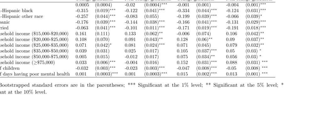
Table 2 Marginal E¤ects on Alcohol Consumption

Dependent variable: Log (drinks per day)

Kernel Regression based estimation OLS based estimation

College graduates Non-college graduates College graduates Non-college graduates

Age 0.0005 (0.0004) -0.02 (0.0004) -0.001 (0.001) -0.004 (0.001)

Non-Hispanic black -0.315 (0.019) -0.122 (0.041) -0.334 (0.044) -0.124 (0.031)

Non-Hispanic other race -0.257 (0.044) -0.083 (0.055) -0.199 (0.039) -0.066 (0.039)

Hispanic -0.176 (0.039) -0.144 (0.038) -0.166 (0.041) -0.131 (0.029)

Married -0.063 (0.041) -0.101 (0.011) -0.171 (0.019) -0.191 (0.018)

Household income ($15,000-$20,000) 0.161 (0.111) 0.133 (0.062) -0.006 (0.074) 0.106 (0.042)

Household income ($20,000-$25,000) 0.108 (0.070) 0.091 (0.043) 0.128 (0.06) 0.09 (0.037)

Household income ($25,000-$35,000) 0.071 (0.042) 0.081 (0.024) 0.071 (0.045) 0.079 (0.032)

Household income ($35,000-$50,000) 0.039 (0.031) 0.025 (0.017) 0.105 (0.037) 0.05 (0.03)

Household income ($50,000-$75,000) 0.005 (0.015) -0.012 (0.017) 0.075 (0.034) 0.056 (0.03)

Household income ( $75,000) 0.033 (0.006) -0.004 (0.016) 0.152 (0.031) 0.088 (0.031)

# of children -0.032 (0.003) -0.023 (0.003) -0.047 (0.008) -0.05 (0.008)

# of days having poor mental health 0.001 (0.0003) 0.001 (0.0003) 0.015 (0.002) 0.013 (0.001)

Using either the nonparametric kernel regression or OLS in the …rst-stage, the

es-timates are similar, and are consistent with the existing literature. For example, like

Cook and Moore (1993) and Manning et al. (1995), I …nd that, other things equal, white

males drink more than blacks and other minorities. Also, drinking is low in the lowest

income bracket (under $15,000 per year), but otherwise drinking tends to decrease as

income increases, particularly among non-college graduates.

4

Conclusions

I propose a method of semiparametrically estimating a binary random e¤ects model using

cross-section data. The functional form of the regression function and the distributions

of the random e¤ects and the remaining error are all nonparametric.

The model is applied to a sample of healthy male adults who are regular drinkers.

Alcohol consumption is speci…ed as a binary random e¤ects model, capturing

individ-ual heterogeneity in health-consciousness. I …nd that health-conscious drinkers consume

about half a drink per day on average, while those who are not consume near or over 2

drinks per day. These estimates are consistent with the typical de…nition of heavy

drink-ing for males. Further, college education is found to be associated with a higher

proba-bility of health-consciousness and a lower level of drinking among heavy drinkers. The

unobserved binary random component capturing individual types is shown to explain a

signi…cant proportion of the otherwise unexplained variation in alcohol consumption.

References

Chen, X., O. Linton and I. Van Keilegom, 2003. Estimation of Semiparametric

Cook, J.P. and M.J. Moore, 1993. Drinking and schooling. Journal of Health

Eco-nomics 12, 411-429.

Dong, Y. and A. Lewbel, Nonparametric Identi…cation of a Binary Random Factor

in Cross Section Data, Boston College Working Paper 707.

Fletcher, M.J., P. Deb and J.L. Sindelar, 2009. Tobacco Use, Taxation and Self

Control in Adolescence. NBER Working Paper 15130.

Manning, G.W., L. Blumberg and L.H. Moulton, 1995. The demand for alcohol:

The di¤erential response to price. Journal of Health Economics 14, 123-148

Reboussin, B.A., E. Songa, A. Shresthab, K. K. Lohmana, and M. Wolfson, (2006)

A latent class analysis of underage problem drinking, Drug and Alcohol Dependence,

83, 199-209

Smith, G.W. and M. Shevin, (2008) Patterns of Alcohol Consumption and Related

Behaviour in Great Britain: A Latent Class Analysis, Alcohol and Alcoholism, 43,