Contest Design: An Experimental Investigation

Munich Personal RePEc Archive

Contest Design: An Experimental

Investigation

Sheremeta, Roman

2009

Online at

https://mpra.ub.uni-muenchen.de/52101/

Contest Design: An Experimental Investigation

Roman M. Sheremeta *

Department of Economics, Krannert School of Management, Purdue University,

403 W. State St., West Lafayette, IN 47906-2056, U.S.A.

March 25, 2009

Abstract

This paper experimentally compares the performance of four simultaneous lottery contests: a grand contest, two multiple prize settings (equal and unequal prizes), and a contest which consists of two subcontests. Consistent with the theory, the grand contest generates the highest effort levels among all simultaneous contests. In multi-prize settings, equal prizes produce lower efforts than unequal prizes. The results also support the argument that joint contests generate higher efforts than an equivalent number of subcontests. Contrary to the theory, there is significant over-dissipation. This over-dissipation can be partially explained by strong endowment size effects. Subjects who receive higher endowments tend to over-dissipate, while such over-dissipation disappears when the endowments are lower. This behavior is consistent with the predictions of a quantal response equilibrium. We also find that less risk-averse subjects over-dissipate more.

JEL Classifications: C72, C91, D72

Keywords: rent-seeking, contest, contest design, experiments, risk aversion, over-dissipation

Corresponding author: Roman M. Sheremeta; E-mail: [email protected]

1. Introduction

Costly competitions between economic agents are often portrayed as contests. Examples

range from college admissions and competition for promotions to global relationships in which

different countries and political parties expend resources to lobby their own interests (Krueger,

1974; Tullock, 1980). The variety of economic situations that can be described as contests has

attracted enormous attention from economic theorists. The main focus of this literature is the

relationship between the setup of rent-seeking contests and the strategic behavior of contestants.

It is well recognized that strategic behavior is sensitive to different contest rules. Therefore,

depending on the objective, a careful design of each contest is required.

Despite the abundance of theoretical work on contest design, no experimental research

has specifically compared alternative contest mechanisms.1 To begin to bridge this gap, this

study investigates and compares the performance of four simultaneous contests: a grand contest,

two multi-prize settings (equal and unequal prizes), and a contest which consists of two

subcontests. Consistent with the theory, we find that the grand contest generates the highest

effort levels among all simultaneous contests. In multi-prize settings, equal prizes produce lower

efforts than unequal prizes. Our results also provide strong empirical support for the argument

that joint contests generate higher efforts than an equivalent number of subcontests. However,

contrary to the theory, we find significant over-dissipation in all contests. This over-dissipation

can be partially explained by strong endowment size effects. Subjects who receive higher

endowments tend to over-dissipate, while such over-dissipation disappears when the

endowments are lower. This behavior is consistent with the predictions of a quantal response

1 _{Several experimental studies looked at the design of rank order tournaments (Orrison et al., 2004; Harbring and}

equilibrium. Finally, there is a strong heterogeneity between subjects and individual expenditures

over time, which is clearly inconsistent with the symmetric pure strategy equilibrium. The

deviations from the symmetric equilibrium can be explained to some extent by differences in risk

preference and probabilistic nature of lottery contests.

A number of theoretical papers have been devoted to the design of an optimal contest that

generates the highest revenue – the total amount of effort expended by the contestants. A common motivation for such research is the objective of various agencies (political parties,

lottery administrators, and economic groups) to maximize earnings by extracting the highest

effort from the contestants. Gradstein and Konrad (1999), for example, provide a rationale for a

multi-stage contest design by endogenizing the choice of contest structure. They show that,

depending on a return to scale parameter of the contest success function, a multi-stage contest

may induce higher effort by the participants than a one-stage contest. In the same line of

research, Baik and Lee (2000) study a two-stage contest with effort carryovers. They

demonstrate that, in the case of player-specific effort carryovers, the rent-dissipation rate

(defined as the ratio of the expended total effort to the value of the prize) increases in the

carryover rate and the rent is fully dissipated with carryover rate equal to one. Finally, Fu and Lu

(2007) investigate the optimal structure of a multistage sequential-elimination contest with

pooling competition in each stage. They demonstrate that the optimal contest eliminates one

contestant at each stage until the finale in which a single winner takes the entire prize.

Overall, it is generally observed in the contest literature that pooling competition

generates higher dissipation rates (Clark and Riis, 1998; Amegashie, 2000; Fu and Lu, 2009;

Moldovanu and Sela, 2006).2 Clark and Riis (1998) show that the income maximizing contest

2 _{For more multiple prize contests see Glazer and Hassin (1988), Barut and Kovenock (1998), and Che and Gale}

administrator obtains the highest rent-seeking effort when, instead of many small prizes, a large

prize is provided. Fu and Lu (2009) demonstrate that the rent dissipation rate increases when the

number of contestants and prizes are scaled up. Therefore, the authors conclude that a grand

contest generates higher revenue than any set of subcontests. Moldovanu and Sela (2006)

investigate a similar problem under the structure of all-pay auctions where all players know their

own abilities and the distribution of abilities in the population. The major finding of Moldovanu

and Sela (2006) is that independently of the number of contestants and the distribution of

abilities, a grand contest generates the highest revenue when the cost function is either linear or

concave. However, it is not always the case that pooling competition generates the highest

efforts. For example, if the contestants have convex costs several prizes may be optimal

(Moldovanu and Sela, 2001; Kräkel, 2006). The non-optimality of a single large prize can also

occur in a contest where players have commonly known but different abilities (Szymanski and

Valletti, 2005).

The empirical evidence for contest design theory is mixed (Szymanski, 2003). Maloney

and McCormick (2000), for example, analyze responses of individual runners to prizes in foot

races. They find a significant relation between the performance and the prize value. Consistent

with Lazear and Rosen (1981), higher prize values cause higher effort levels. Similar to Maloney

and McCormick (2000), Lynch and Zax (2000) examine data on road races in the United States.

They find that the performance increases in response to larger prize spreads. However, when

controlled for ability factor, the impact of the prize spread disappears. The authors thus conclude

that the larger prize spreads produce better performance not because they encourage all runners

To complement the existing empirical studies and to further investigate contest design

problem we conduct a controlled experiment. The experiment is based on the theoretical model

presented in Section 2. Section 3 provides experimental design and testable hypotheses. Section

4 reports the results of the experiment. Section 5 offers alternative explanations for

over-dissipation and heterogeneity observed in the experiment and Section 6 concludes.

2. Theoretical Model

Denote by 𝐶 ≡ 𝐶(𝑁, 〈𝑉_𝑠〉_𝑠=1𝐾 ) a contest with 𝑁 identical risk-neutral players who are

competing for 𝐾 prizes of a common value 𝑉_𝑠, 𝑠 = 1, . . , 𝐾.3 No player may win more than one

prize and there are more players than available prizes. Each player 𝑖 chooses irreversible effort

level of 𝑒_𝑖 to influence the probability of winning. Let Ω_𝑠 be the set of remaining (𝑁 − 𝑠 + 1)

players who have not won one of the (𝑠 − 1) prizes. Then the conditional probability that a

contestant 𝑖 wins the 𝑠-th prize is given by a lottery contest success function:

𝑝𝑖(𝑒𝑖, 𝑒−𝑖; Ω𝑠) =_𝑒 𝑒𝑖

𝑖+∑𝑗∈Ω𝑠𝑒𝑗, 𝑖 ≠ 𝑗 (1)

The efforts are often raised to an exponent term to indicate the sensitivity of a contest.

Our reasons for choosing this specific contest success function is that it is simple enough for

subjects to understand and it is also commonly used in most of the rent-seeking contest literature,

including virtually all of the experimental contest literature. It is important to emphasize,

however, that the simplicity of (1) does not affect the comparative statics predictions of the

theory (Clark and Riis, 1998; Fu and Lu, 2009).

3 _{For theoretical and experimental analysis of heterogeneous agents in lottery contests see Harbring et al. (2007),}

We concentrate our analysis on the symmetric pure strategy Nash equilibrium of the

game. The expected payoff of player 𝑖, 𝐸(𝜋_𝑖), is derived by multiplying player 𝑖’s probability of winning each prize, 𝑝_𝑖(𝑒_𝑖, 𝑒_−𝑖; Ω_𝑠), by its value, 𝑉_𝑠. Since we are considering symmetric

equilibrium the efforts made by other players 𝑖 ≠ 𝑗 can be denoted as 𝑒. Therefore, the

probability that 𝑖 wins the first prize is 𝑒_𝑖/(𝑒_𝑖 + (𝑁 − 1)𝑒). If 𝑖 does not win the first prize, his

conditional probability of winning the second prize is the product of the probability that 𝑖 does

not win the first prize and the probability that he does win the second prize. Applying this

reasoning we can write player 𝑖’s expected payoff as:

𝐸(𝜋𝑖) =_𝑒 𝑒𝑖

𝑖+(𝑁−1)𝑒𝑉1+

(𝑁−1)𝑒 𝑒_𝑖+(𝑁−1)𝑒

𝑒𝑖

𝑒_𝑖+(𝑁−2)𝑒𝑉2+

+_𝑒(𝑁−1)𝑒

𝑖+(𝑁−1)𝑒

(𝑁−2)𝑒 𝑒𝑖+(𝑁−2)𝑒

𝑒𝑖

𝑒𝑖+(𝑁−3)𝑒𝑉3+ ⋯ + ∏

(𝑁−ℎ)𝑒 𝑒𝑖+(𝑁−ℎ)𝑒

𝑒𝑖 𝑒𝑖+(𝑁−𝐾)𝑒𝑉𝐾 𝐾−1

ℎ=1 − 𝑒𝑖

(2)

The expected payoff (2) is based on the assumptions that players are risk-neutral and

have linear costs. However, by relaxing the linearity of costs assumption the comparative statics

predictions of the theory are not affected. In fact, in the derivation of the equilibrium, Clark and

Riis (1998) use a nonlinear cost function 𝑒_𝑖1/𝑟 instead of 𝑒_𝑖, where 𝑟 > (<)1. Differentiating (2)

with respect to 𝑒_𝑖 leads to the equilibrium effort level in the contest 𝐶(𝑁, 〈𝑉_𝑠〉_𝑠=1𝐾 ): 4

𝑒∗ ₌ 1

𝑁∑ 𝑉𝑠(1 − ∑ 1 𝑁−ℎ 𝑠−1 ℎ=0 ) 𝐾

𝑠=1 . (3)

Formula (3) is the building block of the experimental design used in this study. It shows

that the effort level of each contestant depends on the number of contestants, the number of

prizes, the value of prizes, and the ordering of prizes. Especially interesting is the “placement effect”: the contest administrator can increase the effort level (3) by reducing the value of an early prize 𝑉_𝑠 and increasing the value of a later prize 𝑉_𝑠−1 by the same amount. Taking into

account that the revenue collected by the administrator is simply the summation of all individual

efforts, the placement effect justifies the use of a large single prize to maximize the revenue

collected in the contest.

3. Experimental Design and Procedures

3.1. Treatments and Hypothesis

Suppose there are 𝑁 players who are willing to participate in a contest. The administrator

has a budget 𝑉 and he wants to maximize total revenue extracted from contestants. The

administrator must choose how to organize this contest. The simplest way to do this is a

simultaneous move grand contest, in which all players are pooled into one large group with only

one large prize. This type of contest is the baseline treatment of this study.

Treatment GC: The first contest is a grand contest 𝐶₁(𝑁, 𝑉) in which all 𝑁 contestants

are in the same group and they compete for a single prize of value 𝑉. Applying (3) and summing

over all contestants’ efforts, the total revenue collected in 𝐶1 is

𝑇𝑅𝐺𝐶 = 𝑉 (1 −_𝑁1). (4)

If the prize 𝑉 is divisible the administrator must choose how to divide it. He can divide

the prize into several unequal prizes or he can make all prizes equal. The next two treatments

investigate these alternatives.

Treatment UC: In contest 𝐶₂(𝑁, 〈𝑉₁, 𝑉₂〉) all contestants are competing for two unequal

prizes 𝑉₁ =3₄𝑉 and 𝑉₂ = 1₄𝑉. A 3 to 1 ratio of splitting the prize has been proposed by Galton

(1902). Note, that the sum of 𝑉₁ and 𝑉₂ yields the combined prize of value 𝑉. The total revenue

generated by this contest is

Treatment EC: In the third contest, 𝐶₃(𝑁, 〈𝑉₁, 𝑉₂〉), all contestants compete for two

prizes of the same value 𝑉₁ = 𝑉₂ =1

2𝑉. The total revenue collected is derived from formula (3):

𝑇𝑅𝑆𝐶 = 𝑉 (1 −_𝑁1 −_2(𝑁−1)1 ). (6)

Frequently, instead of putting the contestants into one large group, they are split into

several subgroups. In these cases the competition goes on within each group. As a result, the

contest organizer collects the revenue from each subcontest separately.

Treatment SC: This last simultaneous contest treatment consists of two separate and

identical contests 𝐶₄₁= 𝐶₄₂= 𝐶 (1

2𝑁, 1

2𝑉). The SC treatment resembles the EC treatment, but

instead of competition within the same group, contestants are split into two equal size groups 1

2𝑁

and the winner of each group receives a prize value 1

2𝑉. The total revenue collected in both 𝐶41

and 𝐶₄₂ is

𝑇𝑅𝑆𝐶 = 𝑉 (1 −_𝑁2). (7)

Based on the four treatments, we can formalize the following three hypotheses:

Hypothesis 1. Grand contest (GC) generates the highest revenue among all simultaneous

contests.

This hypothesis follows directly from the four treatments listed above. It can also be

derived from Clark and Riis (1998), who showed that an administrator who wishes to maximize

the revenue should combine all of the prizes into one grand prize.

Hypothesis 2. In multi-prize settings, equal prizes (EC) produce lower efforts than

unequal prizes (UC).

This hypothesis comes from the observation that increasing the value of the first prize,

Therefore, the UC treatment should generate higher revenue than the EC treatment, since in the

UC treatment the first prize is 𝑉₁ = 3

4𝑉 while in the EC treatment the first prize is 𝑉2 = 1

2𝑉. Our

final hypothesis is based on a recent study by Fu and Lu (2009), who showed that the joint

contest generates higher revenue than any set of subcontests.

Hypothesis 3. Joint contest (EC) generates higher efforts than equivalent number of

subcontests (SC).

In summary, the four contests can be ranked by the total revenue collected: 𝑇𝑅_𝐺𝐶 >

𝑇𝑅𝑈𝐶 > 𝑇𝑅𝐸𝐶 > 𝑇𝑅𝑆𝐶. If revenue maximization is the objective of the administrator then the

grand contest should be preferred over all other contests, unequal prize splitting should be

preferred over equal prize splitting, and a joint contest should be preferred over two equivalent

subcontests.

3.2. Experimental Procedures

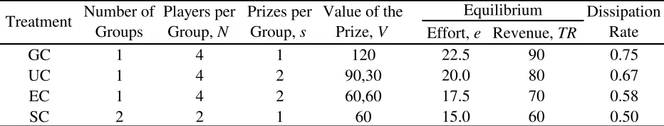
The experiment consists of four different contests. Table 3.1 shows the equilibrium effort

levels, revenue generated by each contest, and dissipation rates, defined as the total expenditures

divided by the total value of the prize, for 𝑁 = 4 and 𝑉 = 120.

Table 3.1 – Experimental Design and Nash Equilibrium Predictions

The experiment used 132 subjects drawn from the population of undergraduate students

at Purdue University. Computerized experimental sessions were run using z-Tree (Fischbacher,

Effort, e Revenue, TR

GC 1 4 1 120 22.5 90 0.75

UC 1 4 2 90,30 20.0 80 0.67

EC 1 4 2 60,60 17.5 70 0.58

SC 2 2 1 60 15.0 60 0.50

Treatment Number of Groups

Players per Group, N

Prizes per Group, s

Dissipation Rate Equilibrium Value of the

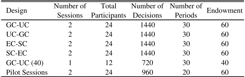
2007) at the Vernon Smith Experimental Economics Laboratory. We ran eleven experimental

sessions with two treatments in each session as in Table 3.2. There were 12 subjects in the lab

during each session. Each experimental session proceeded in three parts. Subjects were given

instructions, available in the Appendix, at the beginning of each part and the experimenter read

the instructions aloud. In the first part subjects made a series of choices in simple lotteries,

similar to Holt and Laury (2002). The second and the third parts of the experiment corresponded

to two out of four treatments. For example, in GC-UC, each subject played in a grand contest for

30 periods, then played for 30 periods in an unequal prize contest. In each period, subjects were

randomly and anonymously placed into a group of 4 players in GC, UC, and EC treatments or

into a group of 2 players in SC treatment.

Table 3.2 – Summary of Treatments and Sessions

At the beginning of each period, each subject received an endowment of 60 experimental

francs. Subjects could use their endowments to expend efforts (place bids) in order to win a

prize. Subjects were informed that by increasing their efforts, they would increase their chance of

winning the prize and that, regardless of who wins the prize, all subjects would have to pay for

their efforts. After all subjects submitted their efforts the computer assigned the winner via a

simple lottery. At the end of each period, the sum of all efforts in the group, the result of the

random draw, and personal period earnings were reported to all subjects. After completing all 60

decision periods, 10 periods were randomly selected for payment (5 periods for each treatment).

GC-UC 2 24 1440 30 60

UC-GC 2 24 1440 30 60

EC-SC 2 24 1440 30 60

SC-EC 2 24 1440 30 60

GC-UC (40) 1 12 720 30 40

Pilot Sessions 2 24 960 20 60

Number of Periods

Design Number of

Sessions

Total Participants

Number of

The earnings were converted into US dollars at the rate of 50 francs to $1. On average, subjects

earned $18 each and this was paid in cash. The experimental sessions lasted for about 70

minutes.

4. Results

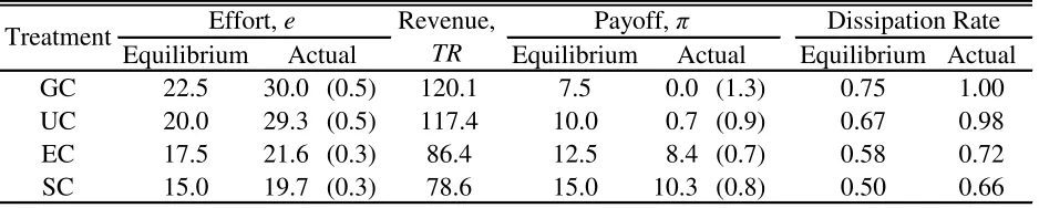
Table 4.1 summarizes average efforts and payoffs over all treatments, and shows that

subjects over-expend effort relative to the risk-neutral Nash prediction. As a result, payoffs are

lower than expected. Note that on average players competing in the grand contest do not earn

any positive payoffs. The dissipation rate is defined as the ratio of the expended total effort

(revenue) to the value of the prize. In the grand contest 100% of the rent is dissipated by 4

players, while only 66% of the rent is dissipated by 4 players in the two subcontests. Actual

dissipation rates are significantly higher than what is predicted by the theory.5

Result 1. Significant over-dissipation is observed in all treatments.

Table 4.1 also reports the total revenue collected in each contest. This revenue can be

calculated by summing up all efforts within a given contest or by multiplying dissipation rate by

the prize value. The data indicates that all four revenues are ranked consistently with the theory.

The revenue collected in the EC treatment is higher than the revenue collected in the SC

treatment. A random-effect regression of effort on the treatment dummy-variable, session

dummy-variables, and a period trend indicates that the revenue difference is significant (p-value

5 _{To support this conclusion we estimated a simple panel regression for each treatment, where the dependent}

< 0.05).6 _{This finding is consistent with Hypothesis 3. The actual difference between the revenue}

collected in the EC and SC treatments is about 8 (=86-78), which is very close to the theoretical

prediction of 10 (=70-60).

Result 2. The equal-prize joint contest generates significantly greater effort and revenue

than the two equivalent subcontests.

Table 4.1 – Average Statistics 7

The next result, which supports Hypothesis 2, is that the revenue collected in the UC

treatment exceeds the revenue collected in the EC treatment. Based on the estimation of a

random-effect model with standard errors clustered at the session level, the difference in

revenues is significant (p-value < 0.05). Although this finding supports Hypothesis 2, the

difference in revenues of 31 (=117-86) is much higher than the theoretical difference of 10

(=80-70).

Result 3. The unequal-prize contest generates significantly greater effort and revenue

than the equal-prize contest.

The grand contest is designed to produce the highest competition from the contestants

and therefore generates the highest revenue for the administrator. Table 4.1 shows that the grand

6 _{When clustering standard errors at the session level, the difference is significant only for the last 15 periods of the}

experiment (p-value < 0.05).

7 _{We also checked for a possible order effect since subjects consecutively played in two of the four possible}

contests. No significant difference was found. In fact, the averages presented in Table 4.1 are almost identical to the averages when we consider only the first treatment in each session. In GC, UC, EC and SC the average efforts without the order effect are 30.2, 29.9, 21.5, and 18.5.

Equilibrium Equilibrium Equilibrium Actual

GC 22.5 30.0 (0.5) 120.1 7.5 0.0 (1.3) 0.75 1.00

UC 20.0 29.3 (0.5) 117.4 10.0 0.7 (0.9) 0.67 0.98

EC 17.5 21.6 (0.3) 86.4 12.5 8.4 (0.7) 0.58 0.72

SC 15.0 19.7 (0.3) 78.6 15.0 10.3 (0.8) 0.50 0.66

Standard error of the mean in parentheses. The total number of observations in each treatment is 1440. Revenue,

TR Treatment Effort, e

Actual

Dissipation Rate Payoff, π

contest indeed generates the highest effort level, the highest revenue, and the highest dissipation

rate. This provides support for Hypothesis 1. Based on the estimation of a random-effect model

with standard errors clustered at the session level, the effort expended in the GC treatment is

significantly higher than the effort expended in the EC treatment (p-value < 0.05) and the SC

treatment (p-value < 0.05). The difference in effort between the GC and UC treatments is

significant only for the last 15 periods of the experiment (p-value< 0.05).8

Result 4. The grand contest generates somewhat higher efforts and revenue than

unequal-prize contest and considerably higher efforts and revenue than either equal-unequal-prize contest or two

equivalent subcontests.

Overall, Results 2, 3, and 4 provide strong empirical support for the theoretical findings

of contest design: the most rent-seeking efforts are obtained when a large prize is provided

instead of several small prizes and the joint contest generates higher revenue than a set of

subcontests. The support for comparative statics comes from aggregate rather than individual

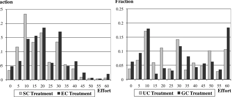
analysis of the data. Figure 4.1a displays the full distribution of efforts made in first 15 periods

of the experiment. It is striking to see that, instead of following a unique pure strategy Nash

equilibrium, subjects’ efforts are distributed on the entire strategy space. In the SC treatment, for example, all efforts should be concentrated at 15, but instead they range from 0 to 60. Similar

behavior is observed in GC, UC, and EC treatments.

Result 5. The actual efforts are distributed on the entire strategy space.

8 _{It is important to emphasize that although the average efforts are similar in both GC and UC treatments, the}

Figure 4.1a – Distribution of Efforts in Periods 1-15

Figure 4.1b – Distribution of Efforts in Periods 16-30

It is often argued that subjects need to get some experience in order to learn how to play

the equilibrium (Camerer, 2003). For that reason, Figure 4.1b displays the distribution of efforts

in final 15 periods of the experiment. The fraction of the equilibrium efforts in the SC and EC

treatments is around 13-16% and the fraction of equilibrium efforts in the GC and UC treatments

is around 4-11%. There is a minor difference between the distribution of efforts in periods 1-15

and periods 16-30. Nevertheless, some learning takes place. The fraction of efforts which are 0 0.05 0.1 0.15 0.2 0.25

0 5 10 15 20 25 30 35 40 45 50 55 60

Fraction

Effort SC Treatment EC Treatment

0 0.05 0.1 0.15 0.2 0.25

0 5 10 15 20 25 30 35 40 45 50 55 60

Fraction

Effort UC Treatment GC Treatment

0 0.05 0.1 0.15 0.2 0.25

0 5 10 15 20 25 30 35 40 45 50 55 60

Fraction

Effort SC Treatment EC Treatment

0 0.05 0.1 0.15 0.2 0.25

0 5 10 15 20 25 30 35 40 45 50 55 60

Fraction

higher than the equilibrium decreases and the fraction of efforts which are lower than the

equilibrium increases with the periods played. This can be seen by the leftward shift of

distributions in Figure 4.1a versus Figure 4.1b (note that there is no leftward shift in the GC

treatment). In Section 5 we provide more formal analysis of the learning trends that occur in our

experiment.

Another argument that is commonly made in the experimental and theoretical literature is

that players may play an asymmetric equilibrium instead of a symmetric equilibrium (Dechenaux

et al., 2006). Although Clark and Riis (1998) do not prove the uniqueness of the pure strategy

equilibrium (3), in our specific case the equilibrium is indeed unique (Szidarovszky and

Okuguchi, 1997; Cornes and Hartley, 2005).9

Figure 4.2 – Average Effort by Subjects in EC-SC and GC-UC Treatments

9 _{Because of experimental design all players are restricted to choose integer effort levels from 0 to 60. Therefore,}

one can look at the 4-player contest as 4-dimensional normal form game with nearly 1.4E+07 possible outcomes. We ran computer simulation to check for all possible pure strategy equlibria and the only one that was found is unique and symmetric. Because of the restriction on the strategy space, in the equilibrium of the GC (EC) treatment two players expend 23 (18) francs and two players expend 22 (17) francs. It is also important to emphasize that because of the concavity of payoff functions the pure strategy equilibrium is also the unique mixed strategy equilibrium. We performed computer simulation for the SC treatment to confirm this.

0 10 20 30 40 50 60

1 7 13 19 25 31 37 43

Average effort

Subject EC Treatment SC Treatment

0 10 20 30 40 50 60

49 55 61 67 73 79 85 91

Average effort

Subject

Figure 4.2 displays the average efforts by all subjects who participated in the experiment.

On the left side each subject is ranked by the average effort he expended in the EC treatment and

on the right side each subject is ranked by the average effort he expended in the GC treatment.

Some subjects never enter the competition and expend zero effort in all periods, while others

expend substantial effort, averaging about 50.10

Result 6. There is a strong heterogeneity in efforts between the subjects.

Uniqueness of the pure strategy equilibrium and findings in Results 1, 5, and 6 produce a

challenge for contest theory. Nevertheless, Results 2, 3, and 4 support the major comparative

static predictions. Why individual behavior is different across subjects is a separate question.

There are many behavioral and demographic factors that may cause these differences. The next

section explores in more detail the possible behavioral and demographic factors that cause

subjects to deviate from the theoretical predictions.

5. Exploring Over-Dissipation

5.1. Quantal Response Equilibrium

Although the comparative statics predictions hold in the experiment, there is a significant

over-dissipation in all treatments (Result 1) which is not captured by the theory. Potters et al.

(1998) conjectured that most subjects are likely to make mistakes. These mistakes add noise to

the Nash equilibrium solution and thus may cause over-dissipation in contest games. We check

this hypothesis by applying a quantal response equilibrium (QRE) developed by McKelvey and

10 _{Evidently, the participants who bid more in the EC treatment are also more likely to bid more in the SC treatment.}

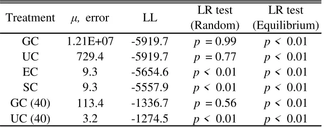
Palfrey (1995). The crucial parameter of this model is the error parameter, μ, which determines

the sensitivity of the choice probabilities with respect to payoffs. The maximum likelihood

estimates of μ for each treatment are shown in the Table 5.1.11 The table also reports the

corresponding value of the likelihood function. The level of mistakes made in the GC and UC

treatments is very high. We cannot reject the random play hypothesis for either of the treatments.

This conclusion stands even when we estimate the model based on the data from the last 15

periods of the experiment. On the other hand, the behavior in the EC and SC treatments can be

captured by the QRE with a reasonable level of mistakes.

Table 5.1 – QRE Computation Based on All Periods

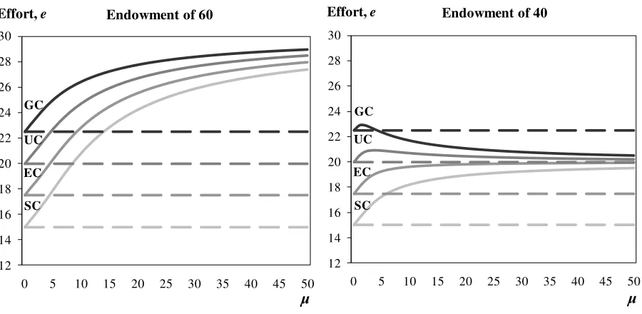
Figure 5.1 illustrates the average effort at the QRE as a function of μ for each treatment.

On the vertical axis we find the average effort for each player. When μ is zero, the behavior is

consistent with the Nash equilibrium. With increasing level of mistakes, all players over-expend

average effort relative to the Nash equilibrium. As players move closer to random play, i.e.,

putting equal weights on each strategy, the average effort approaches 30 (one half of the

endowment). Even without additional computation one can see how the QRE can account for the

over-dissipation in all treatments of the experiment. For example, the average effort of 19.6 in

the SC treatment falls perfectly on the bottom curve around μ≈ 9 (left panel of Figure 5.1).

11 _{The estimation procedure followed Goeree et al. (2002). A more detail description of the estimation procedure is}

available from the author upon a request.

GC 1.21E+07 -5919.7 p = 0.99 p < 0.01

UC 729.4 -5919.7 p = 0.77 p < 0.01

EC 9.3 -5654.6 p < 0.01 p < 0.01

SC 9.3 -5557.9 p < 0.01 p < 0.01

GC (40) 113.4 -1336.7 p = 0.56 p < 0.01 UC (40) 3.2 -1274.5 p < 0.01 p < 0.01 LR test (Equilibrium)

Treatment μ, error LL LR test

It is important to emphasize that computation of QRE is heavily dependent on the initial

endowment which subjects receive to play the contest game. In our experiment, each period all

subjects receive an endowment of 60. Given this endowment, according to the QRE, at each

level of mistakes subjects can only expend effort which is higher than the Nash equilibrium (left

panel of Figure 5.1). Therefore, one may argue that the over-dissipation in contests can always

be explained by the QRE.12 _{However, this argument is not necessarily true because lower}

endowments may lead to under-dissipation relative to the Nash equilibrium prediction. For

example, when the endowment is 40, the QRE predicts that higher level of mistakes in the GC

treatment should result in under-dissipation (right panel of Figure 5.1). The intuition behind this

prediction is straightforward: when subjects have large endowments then their mistakes are more

likely to result in over-dissipation, while small endowments are more likely to result in

under-dissipation.

Figure 5.1 – Average Effort at the QRE

12 _{Bullock and Rutstrom (2007) find that observed behavior in the Tullock-type model of political competition is}

fully captured by QRE predictions. Anderson et al. (1998) develop a theoretical model of the all-pay auction based on the QRE. The model predicts that overbidding in the all-pay auction occurs due to the mistakes and that overbidding should increase with the size of the bidders’ group. Nevertheless, Gneezy and Smorodinsky (2006) found that the over-dissipation in the all-pay auction is independent of the group size in later periods.

SC GC EC UC 12 14 16 18 20 22 24 26 28 30

0 5 10 15 20 25 30 35 40 45 50

Effort, e

μ

Endowment of 60

SC GC EC UC 12 14 16 18 20 22 24 26 28 30

0 5 10 15 20 25 30 35 40 45 50

Effort, e

μ

To make a definite conclusion, we conducted one more session with GC (40) and UC

(40) treatments. This time each subject was given an endowment of 40 instead of 60. We were

very surprised to discover that the average effort in GC (40) treatment indeed fell from 30.0 to

21.6 which is below the Nash equilibrium prediction of 22.5. In the UC (40) treatment, average

effort fell from 29.3 to 21. This finding is a strong support for QRE.13 It is also consistent with

Sheremeta (2008), who conducted one treatment equivalent to the GC treatment. In that study

subjects were given the endowment of 120 francs instead of 60 and as a result the average effort

was 34.1 instead of 30. A strong effect of the endowment on subjects’ behavior can explain why some experimental studies (Schmidt et al., 2005; Shupp, 2004) find less rent-seeking

expenditures than what is predicted by the equilibrium.14

5.2. Risk Aversion

The QRE model can account for the general trend of over-dissipation in the experiment.

However, it cannot explain the heterogeneity in efforts between the subjects (Result 6). In the

experimental literature it is believed that this heterogeneity is mainly caused by heterogeneity of

risk preferences. Previous experimental studies found a significant effect of risk aversion on the

dissipation rate (Miller and Pratt, 1991). In our experiment, rather than estimating risk aversion

from the observed choices in contest games (Goeree et al., 2002; Schmidt et al., 2005), in the

first stage we used a simple lottery to elicit risk aversion from the subjects.

13 _{With the restriction on the endowment, the estimated level of mistakes,} μ, _{also decreased in both treatments (Table}

5.1). However, in the GC (40) treatment we still cannot reject the random play hypothesis.

14 _{In Schmidt et al. (2005) and Shupp (2004) subjects were given a budget which allowed them to bid up to $20}

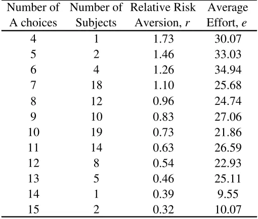
Table 5.2 – Classification of Subjects by Risk Aversion (All Treatments)

Following Holt and Laury (2002), subjects were asked to state whether they preferred

safe option A or risky option B. In the experiment, the majority of subjects chose the safe option

A when the probability of the high payoff in option B was small, and then crossed over to option

B.15 Table 5.2 presents a summary of A choices made by all subjects in the experiment. Risk

neutrality corresponds to the switching point of either 7 or 8 safe choices A. The majority of

subjects show a tendency toward risk-averse behavior. Based on the observed switching point for

each subject, we can estimate their degree of risk aversion.16 To be consistent with other studies

we calculate risk aversion parameters, r, based on the assumption that all subjects have constant

relative risk aversion. The estimates are shown in Table 5.2. Higher r corresponds to lower

number of safe choices A. Conventionally, subjects are considered to be risk-seeking when r > 1.

15 _{Option A yielded $1 payoff with certainty, while option B yielded a payoff of either $3 or $0. The probability of}

receiving $3 or $0 varied across all 15 lotteries. The first lottery offered a 5% chance of winning $3 and a 95% chance of winning $0, while the last lottery offered a 70% chance of winning $3 and a 30% chance of winning $0.

16 _{Note that switching from A to B only gives us an interval of risk aversion coefficient. However, for statistical}

computations we will use a mid-point approximation.

4 1 1.73 30.07

5 2 1.46 33.03

6 4 1.26 34.94

7 18 1.10 25.68

8 12 0.96 24.74

9 10 0.83 27.06

10 19 0.73 21.86

11 14 0.63 26.59

12 8 0.54 22.93

13 5 0.46 25.11

14 1 0.39 9.55

15 2 0.32 10.07

Number of A choices

Number of Subjects

Relative Risk Aversion, r

Risk neutrality corresponds to the case when r = 1. As r decreases, subjects become more

risk-averse and prefer more safe options A.

Theoretical work by Hillman and Katz (1984) showed that risk-averse players should

exert lower efforts than the prediction for risk-neutral players and risk-seeking players should

exert higher efforts. Thus, if risk aversion is a crucial factor for explaining heterogeneity between

the subjects then the efforts expended in the contest should be negatively correlated with the

number of safe choices made. The last column of Table 5.2 displays an average effort

corresponding to the number of safe choices A made by all subjects. Consistent with the theory,

there is significant negative correlation between these two variables. The Spearman's rank

correlation coefficient, ρ, is -0.81 and it is significantly different from zero (p-value < 0.05).

5.3. Lag Dependence and Assessment of the Random Draw

So far, we have discussed several explanations for over-dissipation (Result 1) and

heterogeneity between the subjects (Result 6). Another question that needs to be addressed is

why actual efforts are distributed on the entire strategy space (Result 5). One explanation may

come from the probabilistic nature of lottery contests. The random draw made by the computer

in period t-1 may affect the individual behavior in period t. To capture this dynamic we

estimated several random-effect (RE) models as in Table 5.3. In the estimation we used the data

only from the 8 main sessions. The estimation results were very similar when sing the data from

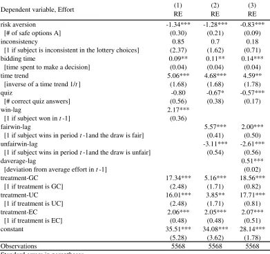
Table 5.3 – Random-Effect Models

Specification (1) is a simple RE regression of individual efforts made in all periods of the

experiment on experimentally relevant explanatory variables. The coefficient capturing risk

aversion is significant and has the expected sign. The variable inconsistency is intended to

capture the subjects who demonstrated inconsistency in their risk preferences. Time spent on

making a decision has a positive effect on over-dissipation. One explanation for this may be that

subjects who take more time to make their decisions are actually confused about what they

should do and therefore they make more mistakes (from section 5.1, more mistakes corresponds

Dependent variable, Effort (1)

RE

(2) RE

(3) RE

risk aversion -1.34*** -1.28*** -0.83***

[# of safe options A] (0.30) (0.21) (0.09)

inconsistency 0.85 0.7 0.18

[1 if subject is inconsistent in the lottery choices] (2.37) (1.62) (0.71)

bidding time 0.09** 0.11** 0.14***

[time spent to make a decision] (0.04) (0.04) (0.04)

time trend 5.06*** 4.68*** 4.59**

[inverse of a time trend 1/t] (1.68) (1.68) (1.78)

quiz -0.80 -0.67* -0.57***

[# correct quiz answers] (0.56) (0.38) (0.17)

win-lag 2.17***

[1 if subject won in t-1] (0.36)

fairwin-lag 5.57*** 2.00***

[1 if subject wins in period t-1and the draw is fair] (0.41) (0.50)

unfairwin-lag -3.11*** -2.61***

[1 if subject wins in period t-1and the draw is unfair] (0.54) (0.56)

daverage-lag 0.51***

[deviation from average effort in t-1] (0.02)

treatment-GC 17.34*** 5.16*** 18.56***

[1 if treatment is GC] (2.48) (1.71) (0.82)

treatment-UC 16.01*** 3.85** 17.71***

[1 if treatment is UC] (2.48) (1.71) (0.81)

treatment-EC 2.06*** 2.05*** 2.07***

[1 if treatment is EC] (0.48) (0.48) (0.51)

constant 35.51*** 34.08*** 28.14***

(5.28) (3.62) (1.78)

Observations 5568 5568 5568

Standard errors in parentheses

* significant at 10%; ** significant at 5%; *** significant at 1%

to higher over-dissipation). We also find that the inverse of a time trend is positive and

significant which suggests that individual learning is taking place and, that with the repetition of

the game, subjects expend lower efforts. The quiz variable is measured by the number of correct

quiz answers (a measure of how well subjects understand the instructions) and is designed to

capture the ability factor.17 Specifications (2) and (3) indicate that subjects who understand the

instructions better expend significantly lower efforts in contests. Therefore, this is another

evidence that the over-dissipation is caused by subjects who make mistakes and who do not

understand the game.

To capture the dynamics of the game we include a win-lag variable. This is a

dummy-variable which takes on the value of 1 if the player won the prize in period t-1 and is 0 otherwise.

In specification (1), this variable has a significant positive effect on effort. One explanation for

this finding is due to the income effect: subjects who won in period t-1 have higher income in

period t and therefore expend higher efforts.18 In specification (2), instead of using win-lag

variable, we use fairwin-lag and unfairwin-lag variables. The fairwin-lag (unfairwin-lag)

variable takes on the value of 1 if subject wins the prize in period t-1 and the random draw in

period t-1 is fair (unfair). The fair draw is defined as a random draw that favors the player whose

effort is higher than the average effort in the group. On the other hand, the unfair draw favors a

player with a low effort. From the estimation, we find that the subjects who expend high efforts

and win raise their efforts in the consecutive period, while the subjects who expend low efforts

and win reduce their efforts in the consecutive period. One may argue that this is simply due to

17 _{Before the actual experiment, subjects completed the quiz on the computer to verify their understanding of the}

instructions. If a subject’s answer was incorrect, the computer provided the correct answer. The experiment started only after all participants had answered all quiz questions.

18 _{It is rather surprising since we tried to avoid this effect by using random payment. It is also possible that subjects}

the fact that subjects who expend higher (lower) efforts in one period are also more likely to

expend higher (lower) efforts in the next period. To address this argument we run specification

(3) in which we include daverage-lag variable. This variable is equal to the difference between

player i’s effort and the average effort in the group in period t-1. From the estimation we find that this variable is indeed significant, i.e., subjects whose efforts are above the average in the

past exert higher efforts in the current period. Even though the magnitudes of fairwin-lag and

unfairwin-lag variables dropped, both variables are still significant. The response to fair and

unfair draw by the subjects is intuitive but it is not rational. Since the nature of winning the

contest is probabilistic, the perception of fair and unfair draw is important in explaining why

subjects vary their efforts across periods and why actual efforts are distributed on the entire

strategy space.

6. Conclusions

In this study we use experimental methods to test several theoretical predictions of

contest design literature. We investigate and compare the performance of four simultaneous

contests: a grand contest, two multi-prize settings (equal and unequal prizes), and a contest

which consists of two subcontests. Consistent with the theory, we find that the grand contest

generates the highest revenue among all simultaneous contests. We also find that in multi-prize

settings, equal prizes produce lower efforts than unequal prizes. Finally, our experiment supports

the argument that joint contests generate higher efforts than the equivalent number of

subcontests.

Although the comparative statics predictions hold in our experiment, consistent with the

over-dissipation of rent (Millner and Pratt, 1989, 1991; Davis and Reilly, 1998; Potters et al.,

1998). Subjects’ heterogeneity can be explained to some extent by differences in risk preferences. Significant over-dissipation can be partially explained by strong endowment size

effects.

We argue that because of the probabilistic nature of lottery contests it is important to

control for lag of winning and misperception of the random draw. Subjects who expend high

efforts and win the prize in period t-1 raise their efforts in the consecutive period, while subjects

who expend low efforts and win in period t-1 substantially decreased their efforts in period t.

These findings are attributed to the misperception of the random draw and they can partly

References

Amegashie, J.A. (2000). Some Results on Rent-Seeking Contests with Shortlisting. Public Choice, 105, 245-253.

Anderson, S.P., Goeree, J.K., & Holt, C.A. (1998). Rent Seeking with Bounded Rationality: An Analysis of the All-Pay Auction, Journal of Political Economy, 106, 828-853.

Baik, K.H., & Lee, S. (2000). Two-Stage Rent-Seeking Contests with Carryovers. Public Choice, 103, 285-296.

Barut, Y., & Kovenock, D. (1998). The Symmetric Multiple Prize All-Pay Auction with Complete Information. European Journal of Political Economy, 14, 627-644.

Bullock, D., & Rutström, E. (2007). Policy making and rent-dissipation: An experimental test, Experimental Economics, 10, 21-36.

Che, Y.K., & Gale, I. (2003). Optimal Design of Research Contests. American Economic Review, 93, 646-671.

Clark, D.J., & Riis, C. (1998). Influence and the Discretionary Allocation of Several Prizes. European Journal of Political Economy, 14, 605-625.

Cornes, R., & Hartley, R. (2005). Asymmetric Contests with General Technologies. Economic Theory, 26, 923-946.

Davis, D., & Reilly, R. (1998). Do Many Cooks Always Spoil the Stew? An experimental analysis of rent seeking and the role of a strategic buyer. Public Choice, 95, 89-115.

Dechenaux, E., Kovenock, D., & Lugovskyy, V. (2006). Caps on Bidding in All-Pay Auctions: Comments on the Experiments of A. Rapoport and W. Amaldoss. Journal of Economic Behavior and Organization, 61, 276-283.

Fischbacher, U. (2007). z-Tree: Zurich Toolbox for Ready-made Economic experiments, Experimental Economics, 10, 171-178.

Fu, Q., & Lu, J. (2007). The optimal multi-stage contest. University of Munich, Working Paper. Fu, Q., & Lu, J. (2009). The Beauty of “Bigness”: on Optimal Design of Multi Winner Contests.

Games and Economic Behavior, forthcoming.

Galton, F. (1902). The Most Suitable Proportion Between The Values Of First And Second Prizes, Biometrika, 1, 385-390.

Glazer, A., & Hassin, R. (1988). Optimal contests. Economic Inquiry, 26, 133-143.

Gneezy, U., & Smorodinsky, R. (2006). All-Pay Auctions – An Experimental Study, Journal of Economic Behavior and Organization, 61, 255-275.

Goeree, J., Holt, C., & Palfrey, T. (2002). Quantal Response Equilibrium and Overbidding in Private-Value Auctions. Journal of Economic Theory, 247-272.

Gradstein, M., & Konrad, K.A. (1999). Orchestrating Rent Seeking Contests. Economic Journal, 109, 536-45.

Harbring, C., & Irlenbusch, B., (2003). An Experimental Study on Tournament Design, Labour Economics, 10, 443-464.

Harbring, C., & Irlenbusch, B., (2005). Incentives in Tournaments with Endogenous Prize Selection, Journal of Institutional and Theoretical Economics, 127, 636-663.

Harbring, C., Irlenbusch, B. Krakel, M., & Selten, R. (2007). Sabotage in Corporate Contests - An Experimental Analysis. International Journal of the Economics of Business, 14, 367-392. Hillman, A.L., & Katz, E. (1984). Risk-Averse Rent Seekers and the Social Cost of Monopoly

Power. Economic Journal, 94, 104-110.

Kräkel, M. (2006). Splitting Leagues, Journal of Economics, 88, 21-48.

Krueger, A.O. (1974). The Political Economy of the Rent-Seeking Society. American Economic Review, 64, 291-303.

Lange, A., List, J.A., & Price, M.K., (2007). Using Lotteries to Finance Public Goods: Theory and Experimental Evidence. International Economic Review, 48, 901-927.

Lazear, E.P., & Rosen, S. (1981). Rank-Order Tournaments as Optimum Labor Contracts. Journal of Political Economy, 89, 841-864.

Lynch, J., & Zax, J. (2000). The Rewards to Running: Prize Structure and Performance in Professional Road Racing, Journal of Sports Economics, 1, 323-340.

Maloney, M.T., & McCormick, R.E. (2000). The Response of Workers to Wages in Tournaments: Evidence From Foot Races, Journal of Sports Economics, 1, 99-123

McKelvey, R., & Palfrey, T. (1995). Quantal Response Equilibria for Normal Form Games. Games and Economic Behavior, 10, 6-38.

Millner, E.L., & Pratt, M.D. (1989). An experimental investigation of efficient rent-seeking. Public Choice, 62, 139–151.

Millner, E.L., & Pratt, M.D. (1991). Risk Aversion and Rent-Seeking: An Extension and Some Experimental Evidence, Public Choice, 69, 81-92.

Moldovanu, B., & Sela, A. (2001). The Optimal Allocation of Prizes in Contests. American Economic Review, 91, 542-558.

Moldovanu, B., & Sela, A. (2006). Contest architecture. Journal of Economic Theory, 126, 70-96.

Morgan, J., & Sefton, M. (2000). Funding Public Goods with Lotteries: Experimental Evidence. Review of Economic Studies, 67, 785-810.

Müller, W., & Schotter, A., (2007). Workaholics and Drop outs in Optimal Organizations. Working Paper, New York University.

Orrison, A., Schotter, A., & Weigelt, K. (2004). Multiperson Tournaments: An Experimental Examination. Management Science, 50, 268-79.

Potters, J.C., De Vries, C.G., & Van Linden, F. (1998). An Experimental Examination of Rational Rent Seeking. European Journal of Political Economy, 14, 783-800.

Schmidt, D., Shupp, R., & Walker, J. (2005). Resource Allocation Contests: Experimental Evidence. Indiana University, Working Paper.

Sheremeta, R.M. (2008). Experimental Comparison of Multi-Stage and One-Stage Contests, Purdue University, Working Paper.

Sheremeta, R.M. (2009). Perfect-Substitutes, Best-Shot, and Weakest-Link Contests between Groups, Purdue University, Working Paper.

Shupp, R. (2000). Single versus Multiple Winner Probabilistic Contests: An Experimental Investigation, Ball State University, Working Paper.

Szidarovszky, F., & Okuguchi, K. (1997). On the Existence and Uniqueness of Pure Nash Equilibrium in Rent-Seeking Games. Games and Economic Behavior, 18, 135-140.

Szymanski, S. (2003). The Economic Design of Sporting Contests, Journal of Economic Literature, 41, 1137-1187.

Szymanski, S., & Valletti, T.M. (2005). Incentive Effects of Second Prizes, European Journal of Political Economy, 21, 467-481.

Appendix

GENERAL INSTRUCTIONS

This is an experiment in the economics of strategic decision making. Various research agencies have provided funds for this research. The instructions are simple. If you follow them closely and make appropriate decisions, you can earn an appreciable amount of money.

The experiment will proceed in three parts. Each part contains decision problems that require you to make a series of economic choices which determine your total earnings. The currency used in Part 1 of the experiment is U.S. Dollars. The currency used in Part 2 and 3 of the experiment is francs. Francs will be converted to U.S. Dollars at a rate of _50_ francs to _1_dollar. At the end of today’s experiment, you will be paid in private and in cash. 12

participants are in today’s experiment.

It is very important that you remain silent and do not look at other people’s work. If you have any questions, or need assistance of any kind, please raise your hand and an experimenter will come to you. If you talk, laugh, exclaim out loud, etc., you will be asked to leave and you will not be paid. We expect and appreciate your cooperation.

At this time we proceed to Part 1 of the experiment.

INSTRUCTIONS FOR PART 1 YOUR DECISION

In this part of the experiment you will be asked to make a series of choices in decision problems. How much you receive will depend partly on chance and partly on the choices you make. The decision problems are not designed to test you. What we want to know is what choices you would make in them. The only right answer is what you really would choose.

For each line in the table in the next page, please state whether you prefer option A or option B. Notice that there are a total of 15 lines in the table but just one line will be randomly selected for payment. You ignore which line will be paid when you make your choices. Hence you should pay attention to the choice you make in every line. After you have completed all your choices a token will be randomly drawn out of a bingo cage containing tokens numbered from 1 to 15. The token number determines which line is going to be paid.

Your earnings for the selected line depend on which option you chose: If you chose option A in that line, you will receive $1. If you chose option B in that line, you will receive either $3 or $0. To determine your earnings in the case you chose option B there will be second random draw. A token will be randomly drawn out of the bingo cage now containing twenty tokens numbered from 1 to 20. The token number is then compared with the numbers in the line selected (see the table). If the token number shows up in the left column you earn $3. If the token number shows up in the right column you earn $0.

Participant ID _________

Decis ion no.

Optio n A

Option B

Please choose A or B

1 $1 $3 never $0 if 1,2,3,4,5,6,7,8,9,10,11,12,13, 14,15, 16,17,18,19,20

2 $1 $3 if 1 comes out of the bingo cage

$0 if 2,3,4,5,6,7,8,9,10,11,12,13,14,15, 16,17,18,19,20

3 $1 $3 if 1 or 2 comes out $0 if 3,4,5,6,7,8,9,10,11,12,13,14,15, 16,17,18,19,20

4 $1 $3 if 1,2 or 3 $0 if 4,5,6,7,8,9,10,11,12,13,14,15, 16,17,18,19,20

5 $1 $3 if 1,2,3,4 $0 if 5,6,7,8,9,10,11,12,13,14,15, 16,17,18,19,20

6 $1 $3 if 1,2,3,4,5 $0 if 6,7,8,9,10,11,12,13,14,15, 16,17,18,19,20

7 $1 $3 if 1,2,3,4,5,6 $0 if 7,8,9,10,11,12,13,14,15, 16,17,18,19,20

8 $1 $3 if 1,2,3,4,5,6,7 $0 if 8,9,10,11,12,13,14,15, 16,17,18,19,20

9 $1 $3 if 1,2,3,4,5,6,7,8 $0 if 9,10,11,12,13,14,15, 16,17,18,19,20

10 $1 $3 if 1,2,3,4,5,6,7,8,9 $0 if 10,11,12,13,14,15,16,17,18,19,20

11 $1 $3 if 1,2, 3,4,5,6,7,8,9,10 $0 if 11,12,13,14,15,16,17,18,19,20

12 $1 $3 if 1,2, 3,4,5,6,7,8,9,10,11 $0 if 12,13,14,15,16,17,18,19,20

13 $1 $3 if 1,2, 3,4,5,6,7,8,9,10,11,12 $0 if 13,14,15,16,17,18,19,20

14 $1 $3 if 1,2,3,4,5,6,7,8,9,10

11,12,13 $0 if 14,15,16,17,18,19,20

15 $1 $3 if 1,2,3,4,5,6,7,8,9,10

INSTRUCTIONS FOR PART 2 YOUR DECISION

The second part of the experiment consists of 30 decision-making periods. At the beginning of each period, you will be randomly and anonymously placed into a group of 4 participants. The composition of your group will be changed randomly every period. Each period, you and all other participants will be given an initial endowment of

60 francs. You will use this endowment to bid for a reward. The reward is worth 120 francs to you and the other three participants in your group. You may bid any integer number of francs between 0 and 60. An example of your decision screen is shown below.

Decision Screen YOUR EARNINGS

After all participants have made their decisions, your earnings for the period are calculated. These earnings will be converted to cash and paid at the end of the experiment if the current period is one of the five periods that is randomly chosen for payment. If you receive the reward your period earnings are equal to your endowment plus the reward minus your bid. If you do not receive the reward your period earnings are equal to your endowment minus your bid.

If you receive the reward: Earnings = Endowment + Reward – Your Bid = 60 + 120 – Your Bid If you do not receive the reward: Earnings = Endowment – Your Bid = 60 – Your Bid

The more you bid, the more likely you are to receive the reward. The more the other participants in your group bid, the less likely you are to receive the reward. Specifically, for each franc you bid you will receive one lottery ticket. At the end of each period the computer drawsrandomly one ticket among all the tickets purchased by

4 participants in the group, including you. The owner of the drawn ticket receives the reward of 120 francs. Thus, your chance of receiving the reward is given by the number of francs you bid divided by the total number of francs all 4 participants in your group bid.

Chance of receiving Your Bid =

the reward sum of all 4 Bids in your group

In case all participants bid zero, the reward is randomly assigned to one of the four participants in the group.

Example of the Random Draw

65 (10 + 15 + 0 + 40). As you can see, participant 4 has the highest chance of receiving the reward: 0.62 = 40/65.

Participant 2 has 0.23 = 15/65 chance, participant 1 has 0.15 = 10/65 chance, and participant 3 has 0 = 0/65 chance of receiving the reward.

After all participants make their bids, the computer will make a random draw which will decide who receives the reward. Then the computer will calculate your period earnings based on your bid and whether you received the reward or not.

At the end of each period, your bid, the sum of all bids in your group, whether you received the reward or not, and the earnings for the period are reported on the outcome screen as shown below. Once the outcome screen is displayed you should record your results for the period on your Personal Record Sheet under the appropriate heading.

Outcome Screen

IMPORTANT NOTES

You will not be told which of the participants in this room are assigned to which group. At the beginning of each period you will be randomly re-grouped with three other participants to form a four person group. You can never guarantee yourself the reward. However, by increasing your contribution, you can increase your chance of receiving the reward. Regardless of who receives the reward, all participants will have to pay their bids.

At the end of the experiment we will randomly choose 5 of the 30 periods for actual payment in Part 2

using a bingo cage. You will sum the total earnings for these 5 periods and convert them to a U.S. dollar payment, as shown on the last page of your record sheet.

Are there any questions?

INSTRUCTIONS FOR PART 3

The third part of the experiment consists of 30 decision-making periods. The rules for part 3 are almost the same as the rules for part 2. At the beginning of each period, you will be randomly and anonymously placed into a group of 4 participants. The composition of your group will be changed randomly every period. Each period you will be given an initial endowment of 60 francs. The only difference is that in part 3, you will use this endowment to bid for two rewards (instead of one reward). The first reward is worth 90 francs and the second reward is worth 30

francs to you and the other three participants in your group. You may bid any integer number of francs between 0

and 60. After all participants have made their decisions, your earnings for the period are calculated in the similar way as in part 2.

If you receive the second reward: Earnings = Endowment + Second Reward – Your Bid = 60+30–Your Bid If you do not receive either reward: Earnings = Endowment – Your Bid = 60–Your Bid

The more you bid, the more likely you are to receive either first or second reward. The more the other participants in your group bid, the less likely you are to receive any reward. Specifically, for each franc you bid you will receive one lottery ticket. At the end of each period the computer drawsrandomly one ticket among all the tickets purchased by 4 participants in the group, including you. The owner of the drawn ticket receives the first reward of 90 francs. Thus, your chance of receiving the first reward is given by the number of francs you bid divided by the total number of francs all 4 participants in your group bid.

Chance of receiving Your Bid =

the first reward sum of all 4 Bids in your group

In case you do not receive the first reward there is a second draw for the second reward. For the second draw computer drawsrandomly one ticket among all the tickets purchased by 3 participants in the group who did not receive the first reward (the participant who received the first reward is excluded from the second draw). The owner of the drawn ticket receives the second reward of 30 francs. Your chance of receiving the second reward is given by the number of francs you bid divided by sum of 3 bids made by the participants who did not receive the first reward.

Chance of receiving Your Bid =

the second reward sum of 3 Bids (made by participants who did not receive the first reward)

Each participant can win at most one reward. In case all participants bid zero, the first and the second reward is randomly assigned to two of the four participants in the group.

Example of the Random Draw

This is a hypothetical example used to illustrate how the computer is making a random draw. Let’s say participant 1 bids 10 francs, participant 2 bids 15 francs, participant 3 bids 0 francs, and participant 4 bids 40 francs. Therefore, the computer assigns 10 lottery tickets to participant 1, 15 lottery tickets to participant 2, 0 lottery tickets to participant 3, and 40 lottery tickets for participant 4. Then, for the first random draw, the computer randomly draws one lottery ticket out of 65 (10 + 15 + 0 + 40). As you can see, participant 4 has the highest chance of receiving the first reward: 0.62 = 40/65. Participant 2 has 0.23 = 15/65 chance, participant 1 has 0.15 = 10/65

chance, and participant 3 has 0 = 0/65 chance of receiving the first reward.

After all participants make their bids, the computer makes a first random draw which decides who receives the first reward. Let’s say that participant 4 has received the first reward. Then, for the second random draw, the computer randomly draws one lottery ticket out of 25 (10 + 15 + 0). Since participant 4 has already received first reward he is excluded from the second draw. Now, as you can see, participant 2 has the highest chance of receiving the second reward: 0.6 = 15/25. Participant 1 has 0.4 = 15/25 chance and participant 3 has 0 = 0/25 chance of receiving the second reward.

To summarize, all participants will make only one bid. After all participants have made their decisions, the computer will make two consecutive draws which will decide who receives the first and the second reward. Regardless of who receives the first and the second reward, all participants will have to pay their bids. Then the computer will calculate your period earnings based on your bid and whether you received either reward.

At the end of each period, your bid, the sum of all bids in your group, whether you received the first reward or not, whether you received the second reward or not, and the earnings for the period are reported on the outcome screen. Once the outcome screen is displayed you should record your results for the period on your Personal Record Sheet under the appropriate heading.

At the end of the experiment we will randomly choose 5 of the 30 periods for actual payment in Part 3

using a bingo cage. You will sum the total earnings for these 5 periods and convert them to a U.S. dollar payment, as shown on the last page of your record sheet.