Munich Personal RePEc Archive
The volatility of consumption and output
with increasing industrialization
Gomme, Paul and Zhao, Yan
16 October 2010
The volatility of consumption and output with
increasing industrialization
Paul Gomme
Department of Economics
Concordia University
[email protected]
Yan Zhao
School of Business
East China University of Science
and Technology
[email protected]
August 2011
Abstract
Consumption is more volatile than output in developing countries while it is less
volatile than output in developed economies. This paper shows that the
relative-ly large home sector in developing economies contributes to this difference, and the
driving force for this difference is technology. Thus this paper suggests that volatile
market consumption is almost inevitable at the start of industrialization, when the
1
Introduction
In the business cycle literature, the notion that consumption is generally less volatile than
output, is commonly known and widely accepted. Implied by the theory of consumption
smoothing and supported by the data, less volatile consumption relative to output seems
commonsense.
This rule, however, is not universally observed in the data. For many developing
countries, such as Argentina, Brazil, Mexico, and South Africa, consumption is more
volatile than output. Recently, this fact has been noticed and the related literature is
growing. For example, Garcia-Cicco et al. (2009) calculate the ratio of the volatility of
consumption to that of output for Argentina, 1900−2005, to be 1.4;Aguiar and Gopinath
(2007) find the same ratio to be 2.01 for Brazil and 1.24 for Mexico, and the average for
developing countries is 1.45. The former attributes the relatively greater volatility of
con-sumption in developing countries to preference shocks, but do not investigate the
corre-sponding impact of the same shocks on developed countries. It cannot be argued that
preference shocks cause the greater volatility of consumption relative to output in
de-veloping countries without first checking whether the same shocks cause the same or
different effects in developed countries. Insofar as the effects are the same, the
differ-ence in relative volatilities remains unexplained. Insofar as they are different, and of the
right size and direction, there may be an explanation, at least to some degree. The same
methodology must hold for any factor proposed as a potential cause of the difference in
relative volatilities, for example, productivity, literacy or mortality, and a check of the
ef-fects on each block, developing and developed, must be undertaken to establish potential
causation.
Aguiar and Gopinath (2007) adopt the right methodology but concentrate on
tech-nology shocks. In their view, techtech-nology shocks are trend-growth related in
will not adjust consumption much because the agent knows that the shock is not
perma-nent, with the expectation that output will return to the long-run trend. By contrast, in
developing counties, the agent will adjust consumption accordingly because the shock
implies a permanent change in output.
This paper seeks to explain the difference in consumption volatility across economies
in general, and between developed and developing economies in particular, by first
ask-ing a fundamental question: What is the principal difference between a developed and a
developing economy, and how is such difference reflected in the data of each? The
prin-cipal difference is that a developed economy, which is generally in an advanced stage of
industrialization, encompasses a proportionally greater market sector, while a developing
economy has a proportionally greater non-market or home sector. Moreover, the
avail-able data for consumption and output generally concentrate on market activity, the home
sector being ignored to a large extent. Indeed, the home sector is evidently an important
component of total output, whether on the household level or the aggregate level. For
example, the U.S. time-use survey indicates that market work and home work constitute
33 and 25 percent of discretionary time for a typical household. On the aggregate level,
Eisner (1988) suggests that household production is between 20 to 50 percent of GNP; more recently,Blankenau and Kose(2007) argue that this ratio is 40 to 50 percent for most
industrialized economies. For its importance on data, more recently,Gomme and Rupert
(2007) argue that
“For the purposes of calibration and measurement, it is useful to include a
home production sector even if the specific questions being studied do not
explicitly call for a home sector.”
The main objective of this paper is to investigate whether the difference in
consump-tion volatility across countries can be explained by the difference in the relative
impor-tance of home sectors. The intuition is straightforward: the home sector in developing
e-conomies. Aggregate consumption, which includes both market produced and home
produced goods, may not be as volatile in developing countries as the data suggest.
The main work concentrates on finding key differences across countries that can affect
relative volatility. The various factors taken into consideration here include differences
in preferences, international linkages and technology. The difference in preferences is
represented by the share of market consumption in total consumption and the elasticity
of substitution between market goods and home produced goods. Sensitivity analysis
shows that the effect of preferences on consumption volatility is ambiguous: the
relation-ship between the volatility of market consumption and preferences is nonlinear. When
the share of market consumption or the elasticity of substitution increases, the volatility of
market consumption first increases and then decreases. This suggests that consumption
tends to be volatile within the moderate range, not at the extremes.
Another notable difference between the developing and developed countries is the
degree of international financial integration. Developed economies have access to world
financial markets with fewer constraints and smaller costs, either because of more reliable
financial systems or because of the large number of financial products available.
Exten-sively discussed, the relationship between financial markets and macroeconomic
volatili-ty is still ambiguous. Mendoza(1994) finds that changes in the volatility of consumption
and output are negligible in response to changes of financial openness. Baxter and
Cruci-ni(1995) find that financial integration increases the volatility of output while decreasing
the volatility of consumption. Gavin et al. (1996) study the sources of macroeconomic
volatility in developing countries over the period 1970−92, and find that there is a
sig-nificant positive association between the volatility of capital flows and output volatility.
This paper contributes to this debate by investigating the relationship between
finan-cial integration and consumption’s relative volatility. The degree of finanfinan-cial integration
is modeled as the ease with which a country’s foreign assets may be adjusted through
monotonically with international financial integration. This result is consistent with
con-ventional wisdom that financial markets help to smooth consumption through lending or
borrowing.
One of the most salient differences between developed and developing countries is
the disparity in total factor productivity, that is the market sector’s productivity relative
to the home sector. Since factors of production, like capital and labor, will flow to the
sec-tor that offers the greatest return (expressed in terms of utility), it is relative productivity,
not absolute productivity, in the market and home sectors that determines the allocation
of factors of production. It is generally believed that the productivity discrepancy
be-tween the two sectors is larger in the developed economies, for two reasons. First, one
characteristic of developed economies is economies of scale, which typically occurs in the
advanced stage of the process of industrialization. Developing countries lag behind in
this process. Second and more important, developed economies characteristically invest
more funds in research and development, the primary source of production
enhancemen-t. Even when measured as a percentage of GDP, the top eight countries are all from the developed group.1
Not only is the discrepancy in productivity levels different across countries, the
tech-nology transmission between sectors is also not the same. It is assumed that techtech-nology
can only be transmitted from a more advanced sector to less advanced sectors, namely
from the market sector to the home sector in this paper. For developed economies,
ad-vanced technology and sophisticated equipment are common in the market sector, and
such equipment is virtually unattainable for households. Thus even when there is
techno-logical innovation in the market sector, it is difficult to adopt such innovation in the home
sector. For developing economies, where domestic workshops are common, the situation
is different; technological innovation in one sector will be applicable to the other sector.
The paper shows that, the less productive the market sector is relative to the home sector,
1According to OECD, the top eight are Israel (4.53%), Sweden (3.73%), Finland (3.45%) Japan (3.39%),
and the stronger the transmission effect, the more volatile market consumption(relative
to market output) will become. Moreover, the volatility of market consumption varies
to a greater extent with technology than with preferences and the international linkage;
further changes to production are the only way to generate more volatile consumption,
which implies that technology is the driving force for excess volatile consumption in
many developing countries.
The structure of the paper is as follows. The next section, Section 2 sets up a two
sector model; Section 3 calibrates the parameters and provides the simulation results for
the benchmark economy; Section 4 undertakes sensitivity analysis, in which differences
in preferences, production and the international linkage are presented and their effects on
the volatility of consumption are analyzed. Section 5 summarizes the conclusions of this
paper.
2
The Economic Environment
2.1
Preferences
In a small open economy, the infinitely lived representative agent derives utility from
streams of a composite goodct, and disutility from workingnt. The agent’s preferences
are summarized by:
E0
∞
∑
t=0
θtU(ct,nt) (1)
θ0=1 (2)
θt+1= β[U(ct,nt)]θt (3)
whereθt is the endogenous discount factor,βis a function of past utility with the
restric-tion that its first-order derivatives are negative,β′ <0. 2 This restriction implies that the
2The endogenous discount factor is to overcome the indeterminacy problem, seeMendoza(1991) and
more people consume, the less patient they become. Any increase in current consumption
reduces the subjective discount weight of all future periods.
In the small open economy literature, the functional form for preferences receives
particular attention. The standard form for utility generally fails to produce a
counter-cyclical trade balance, one of the stylized facts for open economies. The GHH utility,
first proposed byGreenwood et al.(1988), performs better and is widely adopted in open
economy models. Moreover, Chapter 1 shows that, in a two sector model, standard
pref-erences lead to macroeconomic volatility, especially for consumption. For the purpose of
concentrating on consumption volatility in this paper, the GHH form is preferred. GHH
preferences have the form
u(ct,nt) =
[ct−µn
ω
t
ω ]1
−γ
1−γ (4)
in which aggregate consumption ct consists of market goods cmt and home-produced
goodscht, and
ct = [π(cmt )
ρ−1
ρ + (1−π)(ch
t)
ρ−1
ρ ] ρ ρ−1
(5)
ntin equation (4) is the sum of working time in the market sectornmt , and the home sector
nht:
nt =nmt +nht (6)
Finallyµin equation (4) is the weight in preferences on labor supply,ωis the elasticity of
labor supply, andγdenotes risk aversion. In equation (5),πis the weight given to market
consumption, andρis the elasticity of substitution between market produced goods and
home made goods. Accordingly, the functional form ofβis
β(ct,nt) = (1+ct−µn
ω
t
ω )
−b
(7)
2.2
Technology and investment
The production function for each sector has the standard form:
yit =expzit(ki
t)α
i
(nit)1−αi, i =m,h (8)
where in sectori,kitis the capital stock,nit is the labor supply,αiis capital share in output andzit is the sector specific technology shock with mean ¯zi.
Let zt be the 2×1 vector [zmt ,zht]
′
with mean ¯z. Productivity shocks evolve according to,
zt =ν∗zt−1+ (I −ν)∗z¯+ǫt, (9)
where I stands for the identity matrix, and ǫt = [ǫm
t ,ǫht]
′
denotes the error terms with
correlation coefficientξ =corr(ǫtm,ǫth). The matrixνis of the form,
ν=
ρmm ρmh
ρhm ρhh
where diagonal elementsρii denote the technology persistence, off-diagonal elementsρij
stand for the technology spill over from sectorjto sectori. The law of motion for capital in sectoriis
kit+1 = (1−δi)ki
t+xit, (10)
where for sectori, δi is the capital depreciation rate, andxit is investment. As is common in the home production literature, it is assumed that home made products are used only
for consumption. Thus investment can be formed only from market sector products. It
is also assumed that a cost occurs to capital adjustment: the more rapid adjustment, the
greater this cost. Capital adjustment cost is modeled as φ2i(kit+1−ki
t)2, and φi is the the
2.3
Linkage to international markets
In this small open economy, the representative consumer can export goods to accumulate
foreign asset holdings, or import goods to finance domestic spending, with the restriction
that only market sector goods can be exported or imported. Together with the condition
that home produced goods can not be invested, this implies
yht =cht. (11)
It is further assumed that whenever borrowing or lending, this consumer faces a fixed
international interest rater∗. Let tbtdenote the trade balance in periodt, anddt stand for
the foreign asset (or debt) holdings, then
dt+1= (1+r∗)dt +tbt. (12)
Since the ease of lending and borrowing reflects the degree of financial integration, it
is appropriate to employ a cost, which depends on the amount of borrowing or lending,
to represent the financial openness of a country. Specifically, this borrowing or lending
cost is approximated as a quadratic function of trade balance, τ2tb2. Backus et al.(1992) call this cost a trading cost. Whereastbt is the net of exports and imports, this term τ2tb2
is called a financial friction in this paper.
Accordingly, the resource constraint for the market sector is,
cmt +dt+1+xmt +xht =ymt + (1+r
∗
)dt−τ
2tb
2
t −
φm
2 (k
m
t+1−kmt )2−
φh
2 (k
h
t+1−kht)2. (13)
Finally, neither the home country nor the foreign country can play a Ponzi-game,
which implies:
3
Calibration and Simulation
As stated in the introduction, the methodology of this paper concentrates on the
differ-ences between developed and developing countries, to identify the factors which explain
consumption volatility. There is, however, no unanimous agreement on how to
catego-rize a country as either developed or developing. Even in the same group, the level of
development may vary widely. Therefore the difference across groups might become less
apparent if averaged by groups. For this reason, it is, perhaps, more illustrative to focus
on two countries, one representing the developed group and the other representing the
developing group, than to average data from each of the groups. For data convenience
and convention, Canada and Mexico, two typical small open economies, are chosen to
represent each group respectively.3
For the market sector in Canada, the share of labor income is calculated to be 68% from
the year 1961 to 2008. Accordingly, the capital share in production, αm, is set to be 32%.
For Mexico, since there is no income basedGDPdata available, this number is also set as 32%. For the home sector, the data is scant for both countries. It is assumed that the home
sector is more labor intensive, so labor share lies in the range[.68, 1.00]. In particular, the
labor shares in the home sector for both countries are set as 86%, the middle value of this
range, and this suggests that the capital share in home sector is 14%. This value is also
adopted inIngram et al.(2007).
Capital depreciation rates in the market sectors,δm, are calculated to be 2.2% for
Cana-da (see Chapter 1), and 2% for Mexico (seeGarcia-Cicco et al. (2009)). Since capital
for-mation in the home sector comes from the market sector, it is assumed that δm = δh for
simplicity. This symmetric treatment also applies to the capital adjustment cost
param-eters, φm and φh, which are assumed to be equal, and their magnitude is calibrated to
match with the volatility of market investment.
substitution between the two goods, ρ, there are no available measurement. Various
pa-pers estimate that the share is around 40%, while the elasticity is 2 for the United States
(Ingram et al. (2007); Blankenau and Kose (2007)). Canada and United States are both
developed countries, and the two countries share many common consumption habits,
therefore it is reasonable to use the same number for Canada. For Mexico, the market
share in consumption is intuitively smaller. For developing countries, market goods are
not prevalent, and the relative price is high. Nevertheless, it is set to be the same as in
Canada for the benchmark economy, and sensitivity analysis on these two parameters
will be conducted in the following section.
As in most papers in the related literature, the international real interest rate, r∗, is set to be 1 percent, suggesting that β in steady state is 0.99. The parameter ω is set at
1.6, implying that the labor supply elasticity 1/(ω −1) = 1.7. The two parameters, µ
and bare jointly determined to meet two ratios: the fraction of time spent working, and the trade balance to GDP. For time spent working, this is set as 61%, the same for both countries, in which 33% goes to the market sector and 28% is spent in the home sector (see
Benhabib et al.(1991)). For the trade balance ratio, the number is calculated to be 1.6% for
Canada and 1.25% for Mexico. The risk aversion parameter, γ, is widely regarded to lie
in the range of 1 to 2, and it is set to be 1.5, the middle value of this range.
For τ, the financial friction parameter, this is chosen so that the marginal cost τtb is 0.58 percent ofGDPas inBackus et al.(1992). This implies thatτ = tb0.58%/GDP. As mentioned earlier, since this parameter represents one key difference across countries, a reasonable
guess is that it indeed varies from country to country.
To estimate the matrix V describing the technological process, the first step is to find the Solow residuals in the two sectors. Solow residuals in the market sectors can be
ob-tained with the available series of output, capital and hours worked. The Solow residual
in the home sector, however, is virtually impossible to compute for lack of data, especially
first is to estimate the parameters in an AR(1) process of the Solow residuals by max-imum likelihood to match with moments in the data as proposed by McGrattan et al.
(1997). The second is to recover output, the capital stock and hours worked in the home
sector from the first order conditions of the model, and then compute the Solow
residu-al, as was originated byIngram et al. (2007). The third approach is to assume the shock
in the home sector has the same process as that of the market sector as inGomme et al.
(2001). For simplicity, this paper adopts the third approach. Thus, the diagonal elements
in matrixVare identical,ρmm =ρhh.
For the off-diagonal elements, ρmh and ρhm, it is assumed that the technology spill
over effect is asymmetric: technology can only spill from more advanced sectors to less
advanced sectors. The market sector is relatively efficient by assumption, and therefore
there is no spill over from home sector, implying thatρmh =0. In contrast,ρhmrepresents
the spill over effect from the market sector to the home sector, and is assumed to be
pos-itive. It is further assumed that spill overs are only partial, implying that ρhm is within
the range [0, 1.0]. The value of this parameter is to set to match with the consumption
volatility ratio in the market sector. For Mexico, this value is 0.90, and for Canada it is
0.52. It is worth noting that the spill over effect may vary across countries. It is easier for
technology to spill to sectors with similar levels of development, or TFP. In particular, if the gap between the market sector and the home sector is big, this effect will be
limit-ed. Another reason for the stronger transmission effect in emerging countries is the lack
of patent protection. Therefore in emerging economies, it is less costly to adopt the new
technology, which typically developed in the advanced sector. 4 For this reason,ρhmis of
particular interest in the sensitivity analysis. ξ = corr(ǫm,ǫh), and its value is set at 0.6, as suggested byBlankenau and Kose(2007).
The last parameter to be set is the technology level in both sectors, ¯zm, and ¯zh. By
4The transmission effect discussed here should be described aseffective transmissionrather thanpotential
normalizing ¯zh =1, ¯zm represents the relative technology advantage in the market sector. The relative technology advantage varies across countries. For extremely
underdevel-oped economies, where family workshops are being transformed to factories in the early
stage of industrialization, it is expected that relative technology is just above unity. With
the development of technology and the expansion of markets, which are characteristic of
further industrialization, established factories or firms may have additional economies of
scale and the technology advantage will grow. Therefore, it seems plausible that the
rela-tive technology advantage is bigger in developed economies.5 Although it is not possible
to obtain an exact value to conduct the simulation in the benchmark model, the market
sector is set to be three times as productive as the home sector for Canada, and 1.5 times
for Mexico. These values imply that ¯zm = 1.1 for Canada and ¯zm = 0.4 for Mexico. The
relative technology advantage is perceived to represent one of the major differences
be-tween developed and developing countries, and so it is necessary to perform sensitivity
[image:14.612.183.426.439.504.2]analysis in the following section.
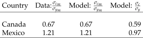
Table 1: Relative Volatility
Country Data:σcm
σym Model:
σcm
σym Model:
σc
σy
Canada 0.67 0.67 0.59
Mexico 1.21 1.21 0.97
The parameter values are summarized in Table 2. With the parameters set in the
benchmark economy, the ratio of market consumption volatility to market output
volatil-ity, σc
σym is 0.53 for Canada, less than the corresponding ratio in the data which is 0.67.
For Mexico, this ratio is 0.803, which is also less than in the data at 1.21, as shown in
Ta-ble1. Nevertheless, the benchmark model generates higher relative volatility in market
5Gollin et al. (2002) examined data for the 1960-90 period for 62 countries and found that the share
of employment in agriculture is negatively correlated with the relative technology advantage. The share of agriculture employment in Mexico is bigger than that in Canada. Agriculture is an analogue to home sector at the start of industrialization, thusGollin et al.(2002)’s result support the claim that ¯zmis greater in
consumption in Mexico, which suggests that adding home sector in the model is in the
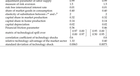
Table 2: Calibration Summary
Parameter Description Canada Mexico
ω labor supply elasticity 1.60 1.60
µ adjustment parameter of labor supply 0.99 0.99
γ measure of risk aversion 1.5 1.5
r⋆
risk free international interest rate 0.01 0.01
π share of market goods in consumption 0.40 0.40
ρ elasticity of substitution betweencm andch 2 2
αm capital share in market production 0.32 0.32
αh capital share in home production 0.14 0.14
δm,δh capital depreciation 0.02 0.02
τ Financial friction parameter 0.36 0.46
ν matrix of technological spill over
0.97 0.00 0.00 0.97
0.95 0.00 0.50 0.95
ξ correlation coefficient of technology shocks 0.6 0.6
¯
zm relative technology advantage of the market sector 1.10 0.40
σm,σh standard deviation of technology shock 0.0063 0.0073
4
Further Discussion
4.1
Sensitivity analysis
As shown in the calibration there is some uncertainty concerning the values of some
pa-rameters either because of a lack of data or of related empirical studies. Notwithstanding
this uncertainty, these parameters were set to some particular ad hoc values for
simu-lation purposes. The ranges for most of these parameters, however, can be determined
from economic theory or stylized facts. Performing a sensitivity analysis gives some feel
for how the results vary with these parameters.
More importantly, some of the parameters vary across countries, and represent some
of the key differences between developed countries and developing countries. As
dis-cussed earlier, the methodology of this paper is to identify these differences and see
which of them contributes to the excessive consumption volatility in developing
coun-tries. Therefore, performing sensitivity analysis is essential to determine the factors which
contribute to the difference in consumption volatility between developed and developing
economies.
Developing countries differ from developed countries in many aspects including
pref-erences, production and international linkages. The difference in preference is
represent-ed by the share of market consumption, π, and the elasticity of substitution, ψ. The
dif-ference in international linkages is embodied inτ, the ease of access to foreign financial
markets. As for different levels of production, this is indicated by ρhm, the technology
transmission from the market sector to the home sector, and ¯zm, the relative technology advantage in the market sector.
The share parameter of market consumption is set at 40 percent for both Mexico and
Canada in the benchmark economy. The home-sector produced goods (and services) in
emerging countries, however, are considered to have a bigger share in total
goods is high. For example, professional day care and old care institutions in some
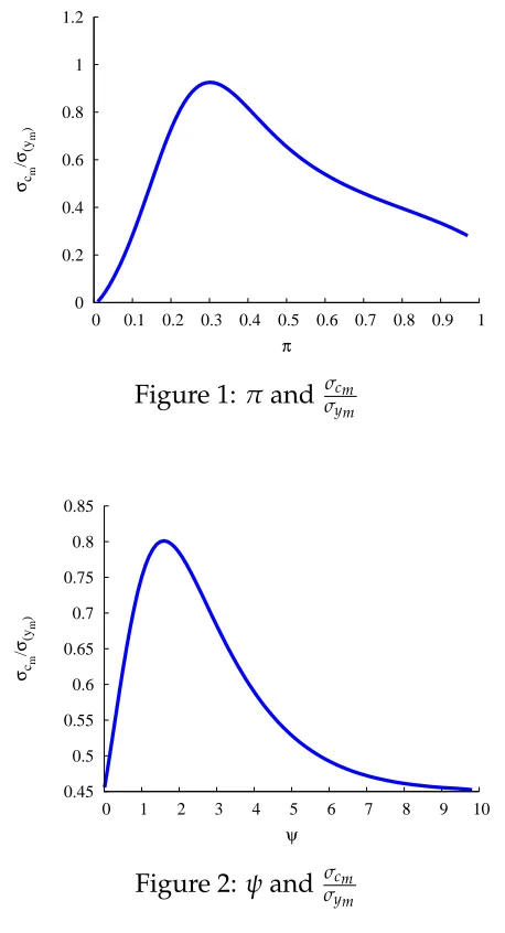
de-veloping countries are rare, and these services are mostly offered at home. π is within
[0.0, 1.0], and the binary relationship between σcm
σym and π is plotted as Figure 1, with all
other parameters fixed in the benchmark model for Mexico. Figure1indicates that as the
share of market consumption increases, its volatility first increases and then decreases.
Specifically, market consumption becomes volatile when this share is around half.
0 0.2 0.4 0.6 0.8 1 1.2
0 0.1 0.2 0.3 0.4 0.5 0.6 0.7 0.8 0.9 1
σcm
/
σ(ym
)
[image:18.612.194.423.221.644.2]π
Figure 1: πand σcm
σym 0.45 0.5 0.55 0.6 0.65 0.7 0.75 0.8 0.85
0 1 2 3 4 5 6 7 8 9 10
σcm
/
σ(ym
)
ψ
Figure 2: ψand σcm
σym
Another factor that represents the difference in preferences is the elasticity of
substi-tution, ψ. The simulation results are presented in Figure2, which also suggests that the
relationship between σcm
exam-ination of Figures 1 and 2 reveals that the maximum consumption volatility σcm
σym is less
than unity, suggesting that the difference in preference is not the main cause for excessive
consumption volatility in developing countries.
τ is the parameter that represents ease of international asset adjustment. Developed
countries can access the international finance markets more easily owing to their more
transparent financial system and sound financial position. Developing countries, on the
other hand, may have to pay an extra cost to enter into the foreign capital market when
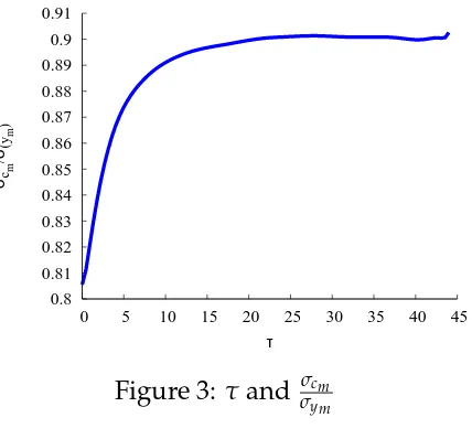
lending or borrowing, particular during a financial crisis. Figure 3 illustrates that the
relative volatility of market consumption increases with the financial friction parameter
τ. However, the effect of financial friction is limited: whenτvaries from 0 to 45, 100 times
as the benchmark value, σcm
σym changes less then 10 percent.
0.8 0.81 0.82 0.83 0.84 0.85 0.86 0.87 0.88 0.89 0.9 0.91
0 5 10 15 20 25 30 35 40 45
σcm
/
σ(ym
)
[image:19.612.204.418.347.546.2]τ
Figure 3: τand σcm
σym
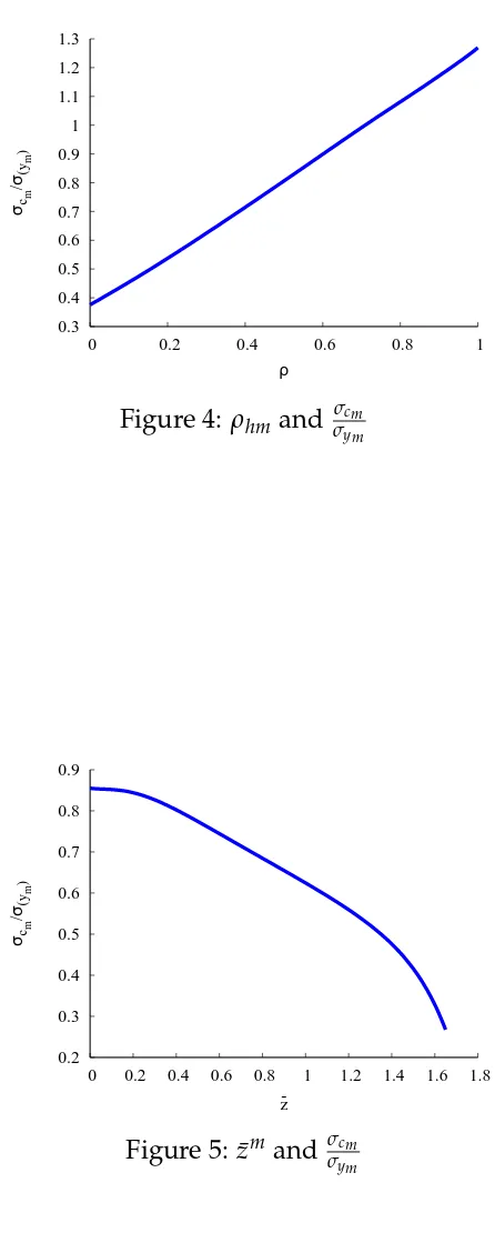
The sensitivity analysis on differences in production is presented in Figure 4 and 5.
Figure 4 indicates that when the transmission effect gets stronger, volatility of market
consumption becomes larger. As discussed earlier, the transmission effect (from the
mar-ket sector to the home sector) is bigger when the productivity gap between sectors is
closer, as it is in developing countries.
0.3 0.4 0.5 0.6 0.7 0.8 0.9 1 1.1 1.2 1.3
0 0.2 0.4 0.6 0.8 1
σcm
/
σ(ym
)
[image:20.612.196.419.125.680.2]ρ
Figure 4: ρhmand σcm
σym
0.2 0.3 0.4 0.5 0.6 0.7 0.8 0.9
0 0.2 0.4 0.6 0.8 1 1.2 1.4 1.6 1.8
σcm
/
σ(ym
)
z
-Figure 5: ¯zm and σcm
investigation reveals that the maximum volatility exceeds unity in Figure4, andσcm
σym varies
more than in Figure1,2and3, implying that a difference in technology is the main cause
for excess consumption volatility in developing countries.
4.2
Benchmark discussion
In Canada, the relative volatility of market consumption is lower because its market sector
is much more important, or dominant. This dominance results from the relative
technolo-gy advantage in the market sector. Market sector’s status calls for particular consumption
smoothing incentives for market consumption. 6
In Mexico, the market sector is not dominant. The main reason for this is the relative
small technology level difference across sectors, i.e., market sector in Mexico has not
de-veloped enough to make home sector trivial. As a result, the market sector consumption
is not smoothed as in Canada.
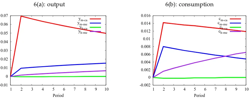
The impulse responses suggest that, for one shock that hits the market sector in
Cana-da, the market sector expands and the home sector shrinks in that yh(ch) decreases. In contrast, for the same shock in Mexico, because of the stronger technology transmission
effect, both sectors expands. Actually, the home sector in Mexico changes more than 20
times in absolute value of the change in Canada.
Also, because of the stronger transmission effect, consumption in Mexico increases to
a greater extent because the agent knows that the positive shock is more persistent. The
consumption change in Canada is small relative to output, reflecting that consumption
smoothing is strong with the expectation the shock is more transitory.
6(a): output -0.01 0 0.01 0.02 0.03 0.04 0.05 0.06 0.07
1 2 3 4 5 6 7 8 9 10
Period ym-ca ym-me yh-ca yh-me 6(b): consumption -0.002 0 0.002 0.004 0.006 0.008 0.01 0.012 0.014 0.016
1 2 3 4 5 6 7 8 9 10
Period
[image:22.612.106.523.80.246.2]cm-ca cm-me ch-ca ch-me
Figure 6: Shock tozm: Output and Consumption
5
Conclusion
This paper offers an explanation for why consumption is generally less volatile than
out-put in developed countries, while it tends to be more volatile than outout-put in developed
countries. By constructing a two sector small open economy model, this paper proposes
for the first time that a relatively large home sector, characteristically found in developing
countries, can explain this phenomenon.
The methodology of the paper has been to extract different factors across countries
and examine which of them generates excessive volatility of market consumption
rela-tive to market output under reasonable conditions. These factors include differences in
preferences, technology and international linkages.
For differences in preferences, the simulation results suggests that their effect on the
relative volatility of consumption is ambiguous. For both the share of consumption and
the elasticity of substitution, the volatility of consumption first increases and then
de-creases, implying that market consumption tends to be most volatile when preferences
for market and home goods are relatively moderate.
For differences in international linkages, this paper refers to frictions in international
results suggests that financial openness helps to smooth market consumption. This effect,
however, is limited in that the variation in consumption volatility is relatively small.
As to the differences in technology, these are embodied in two factors: one is the
mar-ket sector’s relative productivity and the other is the technology transmission effect across
sectors. The sensitivity analysis indicates that the more advanced is a market sector, or the
less effective the transmission effect, both of which correspond to the group of
develop-ing countries, the smoother will be market consumption. The volatility of consumption
exceeds that of output when technology varies, and it is more sensitive to changes in
technology, suggesting that differences in technology are the main cause for excessive
volatility in consumption in some countries.
The conclusion that technology is the driving force for the relative volatility of
con-sumption predicts that volatile market concon-sumption is almost inevitable at the start of
industrialization, when the technology level in the market sector is just above that of the
home sector. With the advancement of the market sector, its consumption will become
less volatile. For this reason, relative volatility of market consumption could be regarded
as an indicator to assess a country’s stage of economic development.
Since excessive volatility leads to a welfare loss, the paper has significant implications.
First, it is implied that the international financial integration helps to smooth
consump-tion. Second and more important, it is also implied that technology enhancement is vital
to reduce the excessive volatility in consumption. Therefore, investment in R&D may be
References
Aguiar, M. and Gopinath, G. (2007). Emerging market business cycles: The cycle is the
trend. The Journal of Political Economy, 115(1):69–102.
Backus, D. K., Kehoe, P. J., and Kydland, F. E. (1992). International real business cycles.
The Journal of Political Economy, 100:745–775.
Baxter, M. and Crucini, M. J. (1995). Business cycles and the asset structure of foreign
trade. International Economic Review, 36(4):821–854.
Benhabib, J., Rogerson, R., and Wright, R. (1991). Homework in macroeconomics:
Household production and aggregate fluctuations. The Journal of Political Economy, 99(6):1166–1187.
Blankenau, W. and Kose, M. A. (2007). How different is the cyclical behavior of home
production across countries? Macroeconomic Dynamics, 11:56–78.
Eisner, R. (1988). Extended accounts for national income and product. Journal of Economic Literature, 26(4):1611–1684.
Garcia-Cicco, J., Pancrazi, R., and Uribe, M. (2009). Real business cycles in emerging
countries. Working paper.
Gavin, M., Hausmann, R., Perotti, R., and Talvi, E. (1996). Managing fiscal policy in latin
america and the caribbean:volatility, procyclicality, and limited credit worthiness. I-ADB working paper.
Gollin, D., Parente, S., and Rogerson, R. (2002). The role of agriculture in development.
The American Economic Review, 92(2):160–164.
Gomme, P., Kydland, F. E., and Rupert, P. (2001). Home production meets time to build.
The Journal of Political Economy, 109(5):1115–1131.
models. Journal of Monetary Economics, 54:460–497.
Greenwood, J., Hercowitz, Z., and Huffman, G. W. (1988). Investment, capacity
utiliza-tion, and the real business cycle. American Economic Review, 78:402–417.
Ingram, B. F., Kocherlakota, N. R., and Savin, N. (2007). Using theory for measurement:
An analysis of the cyclical behavior of home production. Journal of Monetary Eco-nomics, 40:435–456.
McGrattan, E. R., Rogerson, R., and Wright, R. (1997). An equilibrium model of the
busi-ness cycle with household production and fiscal policy.International Economic Review, 38(2):267–290.
Mendoza, E. G. (1991). Real business cycles in a small open economy. The American Economic Review, 81:797–818.
Mendoza, E. G. (1994). Capital Mobility: The Impact on Consumption, Investment, and Growt, chapter 4. Cambridge University Press.