A Self Learning Diagnosis Algorithm Based on Data Clustering

http://dx.doi.org/10.4236/ica.2016.73009

A Self-Learning Diagnosis Algorithm

Based on Data Clustering

Dmitry Tretyakov

“Technekon” Ltd., Moscow, Russia

Received 23 June 2016; accepted 7 August 2016; published 10 August 2016

Copyright © 2016 by author and Scientific Research Publishing Inc.

This work is licensed under the Creative Commons Attribution International License (CC BY).

http://creativecommons.org/licenses/by/4.0/

Abstract

The article describes an approach to building a self-learning diagnostic algorithm. The self-learn- ing algorithm creates models of the object under consideration. The models are formed periodi-cally through a certain time period. The model includes a set of functions that can describe whole object, or a part of the object, or a specified functionality of the object. Thus, information about fault location can be obtained. During operation of the object the algorithm collects data received from sensors. Then the algorithm creates samples related to steady state operation. Clustering of those samples is used for the functions definition. Values of the functions in the centers of clusters are stored in the computer’s memory. To illustrate the considered approach, its application to the diagnosis of turbomachines is described.

Keywords

Self-Learning, Diagnostics, Fault Detection, Clusters, K-Means, Turbomachine, Gas Turbine, Centrifugal Supercharger, Gas Compressor Unit

1. Introduction

The described in the article algorithm and methods can be used for diagnosing a technical object, especially in cases when information about the object is limited. The desired result of the diagnosis is determining the proba-bility of failure and evaluation of changes in the technical condition of the object. The proposed approach was tested by author on various technical objects including turbomachines.

cluster having a specific fault.

Method of separation of object’s states can be chosen after analyzing the features of available data. In [1] fuzzy clustering is used. In [2] a modified method of k-means is considered for clustering and fault diagnosis. Usage of Kohonen self-organizing maps for clustering is described in [3].

In practical application of technical objects a description of its unique fault sometimes is not possible [4]. A diagnostic algorithm may face a new unknown type of fault. At least, a developed diagnostic algorithm should select states of a technical object without faults.

For fault detection signals received from the diagnosed object can be compared with the corresponding values calculated by the object’s model. If the difference between the measured and calculated values (residual) ex-ceeds a predetermined threshold, a fault may occur.

In [5] for estimation of the residuals a Kalman filter is applied. Measurement of distance is used to measure similarity between a new occurred fault and a fault registered in the database. The fault which has the largest be-lief function according to the Dempster-Shafer evidence theory is the most possible fault. The paper [6] presents usage of extended state observer that can be proposed for fault diagnosis without exact knowledge of the diag-nosed object model.

For an object that can be considered as a flat system an approach described in [7] can be used. For the flat system the input signal can be estimated by output signals and their derivatives. In particular, the input signal can be represented as a polynomial function of the output signal and a finite number of its derivatives. For fault diagnosis the gap between the calculated and the measured input value at each time point is estimated.

In [8] an algorithm to detect faults in the sensor is developed. It is assumed that a value of the sensor’s signal transforms from one level to another smoothly and it is caused by a rational reason, such as changing regime of operation. Other behavior of the system may indicate a fault.

Observers can be designed such that they are not sensitive to certain faults while sensitive to other faults in the diagnosed object. This approach is described in [9]. Using a bank of well-designed observers, faults can be detected and isolated simply with the help of the generated residuals.

It is problem to use a set of all possible samples for learning the diagnostics algorithm. In the practical opera-tion of technical objects there are often unforeseen circumstances. The diagnostic algorithm has to use the sig-nals coming from sensors for self-learning. In [10] the learning methods based on association are used for gene-rating new rules from incoming data.

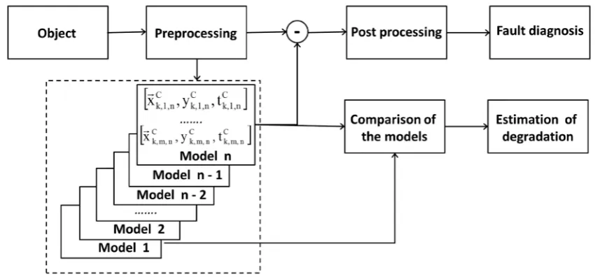
The flow chart of the algorithm discussed in this article is shown inFigure 1. Required information from the object is sent to the diagnostic algorithm. Command signals from controllers, signals from temperature, pressure, vibration and other sensors, position of attenuators, etc. can be used as the information from the object.

Usage of this diagnosis algorithm is restricted to objects that operate at steady state mode during a considera-ble part of their life cycle. For example, it can be applied to turbomachines in power plants or gas compressor

stations, for which the condition usually is determined at steady state operation. The preprocessor selects para-meters related to the steady state operation. In addition, from the received signals it calculates some characteris-tics, such as polytrophic efficiency of the compressor. The self-learning algorithm creates models of diagnosed objects. The models are generated periodically after a specified period of time. For the model identification in-dex n is used in the article.

The object model is a set of functions. A function can describe a whole object or part of the object, or a par-ticular process in the diagnosed object. Comparison of results calculated by different functions with the corres-ponding measurements can provide the fault location. For the function identification index m is used in the ar-ticle.

The processes occurring in the object can be essentially nonlinear. Additionally the processes in the object can have phase transitions. For example, acoustic waves in the combustion system of the gas turbine can be caused by loss of flame stability and phase transition to the unstable combustion. Thus, many functions in a set cannot be described by means of algebraic functions. Therefore, all experimental samples received in the operation of the object are divided into clusters. Then, all functions are defined by their values in the centers of the received clusters. Index k is used in the article for identification of the clusters.

Two approaches to diagnostics are realized in this self-training algorithm. For detection of a fault with rela-tively sharp development the difference between the value calculated by model and the measured value is used. Continuous exploitation of technical object causes its deterioration with relatively smooth development. Com-parison of two models created at the beginning of operation and at the time of diagnostics is used for estimation of the deteriorations.

As an example, usage of this algorithm for turbomachines is described.

2. Model of a Diagnosed Object

n

t and stored in the computer memory. The model consists of a set of statistical functions.

( )

, , ,

m n m n m n

y = f x

Generally, these functions may not have analytical expression.

In practice, for diagnosis of turbomachines this model can include several dozen those statistical functions. Choose of the output variables ym n, depend on method of diagnosis that is planned to use for the object analy-sis.

Input vector xm n, has to define the related output variable ym n, with required accuracy. Input vectors xm n, for different functions fm n, can have different number of members.

Basically, for forming the set of the statistical functions relatively in-depth knowledge about the object is needed. It is assumed that the input vector for each statistical function is known. Usually, in the case of diagno-sis of a technical object the structures of the required functions are known from theory. Otherwise, further study of correlations between the parameters of the object being diagnosed is needed. The study of such correlations is beyond the scope of this article.

It is preferable to form input vector and output variables directly from measured signals that run from sensors. Also in the statistical functions can be used values that are calculated from the measured signals, for example, polytropic efficiency of compressor. In some models, the same value can be an output variable for one of the statistical functions and an input variable for another function.

It is assumed that the diagnosis of the object is performed only for time periods when all the transients are fi-nished and the object is in a stable condition. A group of parameters, which characterize stability of operation of the object, has to be selected. For example, in case of diagnosis of a gas turbine the temperatures along the gas path can be selected.

If within a predetermined period of time the parameters of this group are within the specified range, this time period are considered as one experimental sample indicated by index j.

3. Learning Process

To start diagnosis of the object, the algorithm needs a model of the object. The initial formation of the desired model can be implemented in various ways. The preferred option is the use of a database containing records of signals related to previous work of the analyzed object. If this option is not possible, the self-learning algorithm is able to passively observe the analyzed object until the required set of data samples xj m n_{, ,} ,yj m n_{, ,} ,tj n_,  will

be collected.

For each statistical function m the self-training algorithm divides a set of vectors xj m n, , into clusters with the centers of coordinate xC_{k m n, ,} . The number of clusters determined in advance. For the clustering the well-known method “k-means” can be used.

After determining the coordinates of centers of the clusters x_{k m n}C_{, ,} , the output variable y_{k m n}C_{, ,} and the cha-racteristic time tC_{k m n, ,} are calculated for these centers.

For each cluster k the coefficient of influence w_{j k m n, , ,} of each experimental point j is calculated. The influence coefficient is formed as the product of two coefficients:

, , , , , , , ,

dist age j k m n j k m n j m n

w =w ⋅w

The first coefficient depends on distance between the center of the cluster x_{k m n}C_{, ,} and the experimental

sam-ple x_{j m n, ,} . For the distance the Euclidean determination is used. Then

(

)

, , , , , , , , , 1 exp V m N dist C

j k m n m i k m n i j m n

i

w α x x

=     = − −   

∑

where V m

N is the number of input variables in the statistical function m.

Thus, the experimental point is located far from the center of the cluster has less influence than the experi-mental point, which is located closer.

The second coefficient depends on the period of time between the recording of the experimental point and carrying out clustering:

(

)

(

)

, , exp ,

age M

j m n m n j n

w = −β t −t ,

where M n

t is the time when the model is created and clustering take place.

Thus, the last measurement has a greater influence than measurements in previous time period. The coefficients α_m and β_m are used for the algorithm tuning.

After repair or upgrade of the diagnosed object, the coefficients α_m and β_m can be temporarily increased for an accelerated training the algorithm.

The value of the output variable at the center of the cluster is calculated by polynomial regression function. In particular, the linear regression function can be tested for use.

, , ,

, , , , ,

1

V m

i k m n N

C C

k m n i k m n i

y a x

=

=

∑

The value of the coefficients in the regression function is estimated by the method of least squares taking into account the influence coefficients.

Thus, the coefficients a_{i k m n, , ,} can be found from the following equation:

2 , , , , , , , , , , , 1 1 , , , 0 S V n m N N

j k m n i k m n i j m n j m n

j i

i k m n

w a x y

a = =

 _{ }  ∂ _{ } − =       ∂ _{ } 

∑

∑

where S n

N is number of samples that is used for forming the model n. Then the output variables at the center of the clusters are calculated.

, , , , 1

, ,

, , , 1

S n

S n N

j k m n j n j

C k m n _N

j k m n j

w t

t

w

=

=

=

∑

∑

Finally, information about the centers of the clusters C_{, ,} , C_{, ,} , C_{, ,} k m n yk m n tk m n

 

x  is stored in the computer's memo-ry. Information about the used set of the experimental samples is not stored.

When the self-learning algorithm make a diagnosis of the object new experimental samples are collected in the computer’s memory. The current set of the cluster’s centers C_{, ,} , C_{, ,} , C_{, ,}

k m n yk m n tk m n

 

x  has to be added to the set of new experimental samples _x_{j m n, , +1},y_{j m n, , +1},t_{j n, +1}_ as additional samples.

Then, the procedure of clustering is repeated and the new information about the centers of the clusters

, , 1, , , 1, , , 1

C C C

k m n+ yk m n+ tk m n+

 

x  is stored in the memory.

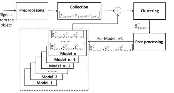
On Figure 2 a flow chart of the learning process of the algorithm is shown. The preprocessing module gene-rates experimental samples from the continuously incoming signals from the diagnosed object. When the num-ber of samples in the set reaches a predetermined numnum-ber, the training process begins.

The generated set of the experimental samples is added to the information of the model with index n. The clustering is curried out and coordinates of new cluster centers x_{k m n}C_{, , +1} are estimated. The post-processing module estimates the output variable y_{k m n}C_{, ,+1} and characteristic time t_{k m n}C_{, , +1} at the cluster centers. Finally, the information of new model with index n+1 is stored in memory of the computer.

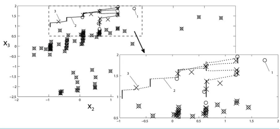
In Figure 3 the example of retraining of algorithm is shown. The algorithm was used for permanent monitor-ing a gas compressor unit. One of the parts of the gas compressor unit was a centrifugal supercharger. For diag-nosis of faults in the centrifugal supercharger several statistical functions were used. One of them was function of pressure drop on an entrance converging cone from the rotational speed of a shaft, inlet temperature, inlet and outlet pressure. Thus, the centers of clusters have been located in 4-dimensional space.

In Figure 3 its 2-dimensional projection is shown, where x₂ is inlet temperature and x₃ is inlet pressure. All values in Figure 3 are given in the normalized form.

The previous clusters centers are marked with markers in the form of a ring (1). Then the monitored gas com-pressor unit work during long period of time. Coordinates related to this work are marked by points (2). All coordinates related to this work are located in a limited area indicated by the dashed line in the upper left corner of Figure 3. The same area is displayed separately in larger scale in the bottom right corner onFigure 3. Then positions of the new centers of clusters were calculated by the technique described earlier. Positions of the new centers of clusters are marked with markers in the form of a cross (3). The algorithm changed the positions of the centers of the clusters only in the area where the work of gas compressor unit took place. The centers located far from this area have not changed their position.

Figure 3. An example of forming a new set of the cluster centers.

4. Diagnosis

Fault diagnosis can be started after the formation of the model of the diagnosed object consisting of sets of clus-ter cenclus-ters. First, the influence coefficients are estimated. The cenclus-ters of clusclus-ters, which located closer to a new measured sample, and were created later have a greater influence, than the centers of clusters located further and were created earlier.

The equations are similar to the previous ones.

, , , , , ,

dist age k m n k m n k m n

w =w ⋅w

(

)

, , , , , , 1 exp V m N dist C

k m n m i m i k m n

i

w α x x

=     = − −   

∑

where x_{i m,} is the input parameters for function f_m.

(

)

(

)

, , exp , ,

age C

k m n m k m n

w = −β t−t ,

where t is time, when diagnosed sample was received.

Then the coefficients a_{i m n}C_{, ,} can be found from the following equation:

2 , , , , , , , , , 1 1 , , 0 C V m m N N

C C C

k m n i m n i k m n k m n C

k i

i m n

w a x y

a = =

 _{ }  ∂  _{ − } ₌     ∂ _{ } 

∑

∑

where C m

N is number of clusters that used for description of function f_m.

Finally, the output value of the function f_m is calculated for the new received sample:

, , , , 1 V n N C m n i m n i m

i

y a x

=

=

∑



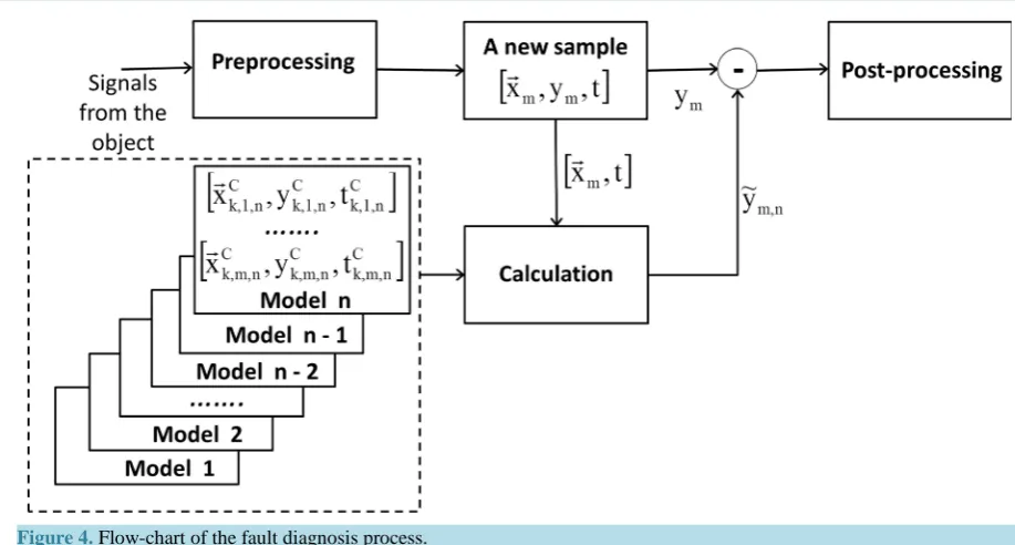
If the difference between the calculated value y_{m n,} and the corresponding measured value exceeds a deter-mined threshold, then a fault can take place.

The flow chart of the described algorithm of fault diagnosis is shown in Figure 4.

In certain cases for fault diagnosis it is rational to use complex criterion, which is formed from various ∆y_m

Figure 4. Flow-chart of the fault diagnosis process.

For diagnostics of the gas turbine the functions which count a difference of temperatures measured by various thermocouples located downstream from the turbine were used.

1

ˆ l l l

T T y

T

+

−

= ,

where T_l and T_l+1 are temperatures measured by adjacent thermocouples, Tˆ is the average temperature after the turbine.

The input parameters of this function are the average temperature after the turbine and the rotation speed of the turbine shaft.

The value K_T was used as a criterion of fault detection in the combustion system of the gas turbines.

(

)

1 TC N

T l l

l

K y y

=

=

∑

where N_TC—number of the thermocouples located after the turbine.

Change of criterion of K_T is shown in the top part ofFigure 5. During long time before the process shown inFigure 5, the gas turbine worked without problem and the criterion K_T was relatively low. Then the crite-rion K_T has dramatically increased, and the diagnosed gas turbine has been stopped after a while. Survey of the stopped gas turbine has shown that the nozzles of the combustors have been destroyed. Obviously, the ab-normal shift of a flame from the ab-normal combustion zone upstream into nozzles has led to their burnout.

For comparison, change of one more criterion of K_V is shown in the lower part ofFigure 5. This criterion is based on a function which calculates the root-mean-square vibration of the turbine. The root-mean-square vibra-tion has been described as a funcvibra-tion of the rotavibra-tion speed of the turbine shaft and its output power.

In addition, the algorithm can be used for estimation of change of technical condition of the diagnosed object caused by its degradation and reduction of its resource. For this estimation several suitable functions have to be chosen. For example, for estimation of degradation of the centrifugal supercharger its polytropic efficiency can be calculated.

One or several sets of constant input parameters for these functions are established. Output values have to be calculated by two models created in different time points.

Figure 5. Criteria related to temperature distribution after turbine and vibration of gas turbine.

efficiency has to be calculated by the next model from the same established values. Reduction of calculated val-ue of polytropic efficiency characterizes deterioration in technical condition of the diagnosed centrifugal super-charger.

5. Conclusion

General information about the diagnosed object is necessary for the proposed algorithm. Numerical parameters of the diagnosed object can be defined at self-learning. The algorithm can be used for diagnosis of significantly non-linear objects. Difference between calculated by the algorithm values and corresponding measured values detects faults. The choice of the suitable functions included in the object model can help with definition of the place of fault. Comparison of the models created in different time points estimates the deterioration in a condi-tion of object caused by long operacondi-tion.

References

[1] Wang, Z., Zhao, N., Wang, W., Tang, R. and Li, S. (2015) A Fault Diagnosis Approach for Gas Turbine Exhaust Gas Temperature Based on Fuzzy C-Means Clustering and Support Vector Machine. Mathematical Problems in Engineer-ing, 2015, Article ID: 240267, 11 p.

[2] Jiang, L., Cao, Y., Yin, H. and Deng, K. (2013) An Improved Kernel K-Mean Cluster Method and Its Application in Fault Diagnosis of Roller Bearing. Engineering, 5, 44-49. http://dx.doi.org/10.4236/eng.2013.51007

[3] Katunin, A., Amarowicz, M. and Chrzanowski, P. (2015) Faults Diagnosis Using Self-Organizing Maps: A Case Study on the DAMADICS Benchmark Problem. Proceedings of the 2015 Federated Conference on Computer Science and Information Systems, ACSIS, 5, 1673-1681. http://dx.doi.org/10.15439/2015F26

[4] Moshou, D., Natsis, A., Kateris, D., Pantazi, X., Kalimanis, I. and Gravalos, I. (2014) Fault Detection of Fuel Injectors Based on One-Class Classifiers. Modern Mechanical Engineering, 4, 19-27.

http://dx.doi.org/10.4236/mme.2014.41003

[5] Wei, X., Guo, K., Jia, L., Liu, G. and Yuan, M. (2013) Fault Isolation of Light Rail Vehicle Suspension System Based on D-S Evidence Theory and Improvement Application Case. Journal of Intelligent Learning Systems and Applications, 5, 245-253. http://dx.doi.org/10.4236/jilsa.2013.54029

[6] Lin, P., Ye, D., Gao, Z. and Zheng, Q. (2012) Intelligent Process Fault Diagnosis for Nonlinear Systems with Uncer-tain Plant Model via Extended State Observer and Soft Computing. Intelligent Control and Automation, 3, 346-355. http://dx.doi.org/10.4236/ica.2012.34040

Satisfaction Approach. International Journal of Applied Mathematics and Computer Science, 23, 171-181. http://dx.doi.org/10.2478/amcs-2013-0014

[8] Liu, Y., Yang, Y., Lv, X. and Wang, L. (2013) A Self-Learning Sensor Fault Detection Framework for Industry Moni-toring IoT. Mathematical Problems in Engineering, 2013, Article ID: 712028, 8 p.

[9] Sobhani, M. and Poshtan, J. (2012) Fault Detection and Insolation Using Unknown Input Observers with Structured Residual Generation. International Journal of Instrumentation and Control Systems, 2, 1-12.

http://dx.doi.org/10.5121/ijics.2012.2201

[10] Kaimal, L. and Metkar, A.G.R. (2014) Self-Learning Real Time Expert System. International Journal on Soft Compu-ting, Artificial Intelligence and Applications, 3, 13-25. http://dx.doi.org/10.5121/ijscai.2014.3202

Submit or recommend next manuscript to SCIRP and we will provide best service for you:

Accepting pre-submission inquiries through Email, Facebook, LinkedIn, Twitter, etc. A wide selection of journals (inclusive of 9 subjects, more than 200 journals) Providing 24-hour high-quality service

User-friendly online submission system Fair and swift peer-review system

Efficient typesetting and proofreading procedure

Display of the result of downloads and visits, as well as the number of cited articles Maximum dissemination of your research work