A Machine Learning Approach to Predicting the Employability of a Graduate

(1)

A Machine Learning Approach to Predicting the

Employability of a Graduate

Masego Modibane

A dissertation submitted to the Faculty of Commerce, University of Cape Town, in partial fulfilment of the requirements for the degree of Master of Philosophy.

January 3, 2019

MPhil in Data Science specialising in Financial Technology, University of Cape Town.

University

of

Cape

(2)

The copyright of this thesis vests in the author. No

quotation from it or information derived from it is to be

published without full acknowledgement of the source.

The thesis is to be used for private study or

non-commercial research purposes only.

Published by the University of Cape Town (UCT) in terms

of the non-exclusive license granted to UCT by the author.

University

of

Cape

(3)

Declaration

I declare that this dissertation is my own, unaided work. It is being submitted for the Degree of Master of Philosophy to the University of Cape Town. It has not before been submitted for any degree or examination.

Masego Modibane

(4)

Abstract

For many credit-offering institutions, such as banks and retailers, credit scores play an important role in the decision-making process of credit applications. It becomes difficult to source the traditional information required to calculate these scores for applicants that do not have a credit history, such as recently graduated students. Thus, alternative credit scoring models are sought after to generate a score for these applicants. The aim for the dissertation is to build a machine learning classifica-tion model that can predict a students likelihood to become employed, based on their student data (for example, their GPA, degree/s held etc). The resulting model should be a feature that these institutions should use in their decision to approve a credit application from a recently graduated student.

(5)

Acknowledgements

I would like to thank my parents, Rapula and Sarah, and the rest of family, espe-cially my grandaunt Granny, for their continued support in the furthering of my education.

I would like to thank Co-Pierre Georg for his belief in - and supervision over this project.

I would like to thank Allan Davids for the help with shaping this dissertation to what it is today.

I would like to thank Sanlam Investments for funding my Masters degree. I would like to thank DataFirst for access to the data used in the project.

(6)

List of Figures

3.1 Data preprocessing procedure performed on theSouth Africa - Grad-uation Destination Survey 2012(2015) data before model testing . . . . 9 3.2 Skeleton of the multi-layer feedforward neural network model. . . . 15 3.3 A general view of a bagged decision tree model . . . 16 3.4 General structures of Receiver Operating Characteristic (ROC) Curves 21 4.1 Neighbour distance plot of theSouth Africa - Graduation Destination

Survey 2012(2015) survey data . . . 24 4.2 Property plot comparison of question 2.1 and 3.3 of South Africa

-Graduation Destination Survey 2012(2015) data. . . 26 4.3 Property plot comparison of question 3.3 and 3.3.2 ofSouth Africa

-Graduation Destination Survey 2012(2015) data. . . 27 4.4 Property plot of question 3.4.13 answer:f ofSouth Africa - Graduation

Destination Survey 2012(2015) data . . . 29 4.5 Property plot of question 3.4.6 ofSouth Africa - Graduation Destination

Survey 2012(2015) data . . . 30 A.1 Basic example of a decision tree classifying between the classesMale

orFemale . . . 45 A.2 Basic structure of a decision tree algorithm . . . 45 B.1 Graph of the Accuracy of prediction against the number of variables

included in the model . . . 46 B.2 Property plot comparison of question 3.4.11 and options a,b,c,d and

f of theSouth Africa - Graduation Destination Survey 2012(2015) data . 51 B.3 Property plot comparison of question 3.4.10 and options a,b, and c

of theSouth Africa - Graduation Destination Survey 2012(2015) data . . 52 B.4 Property plot comparison of question 2.1 and question 2.4.1 of the

South Africa - Graduation Destination Survey 2012(2015) data. . . 53 B.5 Property plot comparison of question 3.3 , 3.3.2, 3.3.3 and question

3.3.4 of theSouth Africa - Graduation Destination Survey 2012(2015) data 54 B.6 Property plot comparison of question 3.4.1.1 , 3.4.3, 3.4.4 and

ques-tion 3.4.6 of theSouth Africa - Graduation Destination Survey 2012(2015) data . . . 55 B.7 Property plot comparison of question 4.1, 4.1.3, 4.1.6, 4.1.4.4 and

question 4.1.5b of the South Africa - Graduation Destination Survey 2012(2015) data . . . 56

(8)

B.8 Prediction accuracy of thek-Nearest Neighbours model at different values of nearest neighbours. . . 58 B.9 Variable Importance plot of the top 10 variables used for the Bagged

decision tree model . . . 60

(9)

List of Tables

3.1 Confusion matrix with a binary classification for the case of predict-ing Employment. . . 20 4.1 Performance Results of the test data on the differently trained

ma-chine learning models . . . 33 4.2 Performance Results of the test data on the top 3 machine learning

algorithms as per the results in table 4.1 . . . 34 4.3 Summary of the changes in the value of the performance measures

when a stress test is performed on the top 3 machine learning models 35 A.1 Advantages and Disadvantages of Classification Decision Trees . . . 44 B.1 Table of the most important variables, in order of importance, as per

the backward selection process. . . 50 B.2 Table of parameters used in machine learning algorithms . . . 57 B.3 Variable Importance Table for Adaptive boosting model. . . 59

(10)

Chapter 1 Introduction

Credit scores play a vital role in the decision-making process of granting consumer credit because they assist in evaluating the financial risk of lending to a particular client. Thomaset al.(2017) define credit scores as a set of decision models which determines who will get credit and how much credit they should get. There is an abundance of research available on credit scoring models built on machine learning algorithms.Baesenset al.(2015) brilliantly summarise the literature available. The article also provides an extensive comparison of these machine learning algorithms. Alternative methods of credit scoring should be considered where there is mul-tiple sources in which individual data can be collected and used to get a better view of the behaviours of the individual. Information about a candidate is now more eas-ily accessible and needs to be included in models that can provide more access to financial products. Transunion, a consumer credit reporting agency, have recently introduced an alternative credit scoring product1. The product aims to provide a more holistic view of the South African consumer to a potential lender. This can lead to more South Africans being considered for loans that they can afford.

The scope of this dissertation is to build an index2that will use university stu-dent data to predict employability after graduation. The intention of this index is to act as a supplement to an existent credit application score model, as opposed to a behavioural scoring model. The resulting model seeks to improve a recent grad-uates probability of obtaining credit and access to other products and services that need a credit score. This aim is in support of the vision set out by the South African Treasury on financial inclusion in South Africa(Achieving Effective Financial Inclusion in South Africa: A Payments Perspective,2014).

The ideal data set for this kind of classification model would include informa-1_{The type of data used is not disclosed but is said to benefit the consumer in the eyes of the} lender (TransUnions New CreditVision Model Uses Alternative and Trended Data to Better Predict Credit Risk, Providing Millions of South Africans with More Opportunities to Gain Access to Credit,2018)

2_{We will be using}_index_and_{classification prediction model}_{interchangeably throughout the} discus-sion

(11)

Chapter 1. Introduction 2

tion about the candidates grade point average (GPA), age, highest degree obtained, type of high school education as well as the candidates assessment marks and their university societal participation. This kind of data can be tracked by the higher ed-ucation institutions at different levels of interaction with the candidate. TheSouth Africa - Graduation Destination Survey 2012(2015) survey data provides us with most of these aformentioned variables in the form of questions asked in the survey. The data also provides an indication of whether the candidate is employed or not. The data is collected from a survey done on the 2010 cohort of graduates from four of the Western Cape Universities. The aim of the survey was to gauge graduate em-ployment (and unemem-ployment). It focussed on various aspects of the graduates path to their employment status as well as the future steps of the graduate. Further discussion of this survey data is in theData description sectionof Chapter3.

According to the South African National Credit Regulations of 2006, approved credit institutions that need the student data mentioned can get the information by requesting for the data from the candidates educational institution/s(Mpahlwa, 2006)3. However, only once consent has been given by the candidate.

Our research approach is to investigate numerous machine learning algorithms across different domains that could be applicable to a case of binary classification. Credit scoring literature deals mostly with regression problems but could easily be extended to classification problems given the outcome of the original regressed score. The literature for alternative credit scoring is a relatively new field and it poses more difficult to find relevant articles. The target with this dissertation is to add to this literature. After investigating a number of machine learning models and performance measures used in both general classification prediction and in credit scoring, we selected 9 models that will be trained and tested on 5 performance measures through a two-stage testing procedure. The first stage of testing used a data set that only has the most important variables forEmployabilityprediction ac-cording to the backward selection process, a feature selection method discussed in more detail in Chapter3. The data set is then divided into a training and test set. All models are then trained with the training set from the abridged data set and tested using the test data set. The top 3 best performing models are then selected to enter the second stage of testing. The second stage applies a stress-testing en-vironment. A new data set consisting of all the other variables that were not seen as important forEmployability prediction by the feature selection method is now used. The data set is then also divided into a training and test set. The models are re-trained on this new data set and tested. The best prediction model is found to be aBagged decision treeaccording to the performance results of both stages.

(12)

Chapter 1. Introduction 3

ever, theAdaboostmodel is a very close second. Surprisingly, all models performed extremely well on all measures chosen at the first stage of testing. However, the performance declined at the second stage of testing. This should be expected as the variables used where not originally seen as important in predictingEmployability. The differences between the model performances were tested for statistical signif-icance. It is found that the models still were able to predict anEmployed test data point correctly. Yet, they did not fair as well in predicting anUnemployedtest data point. Thus, all other measures that involve the (mis)classifying ofUnemployeddata points observed significant differences in their performances

The rest of the dissertation is setup as follows;

• Chapter2provides a discussion of the literature review that focussed on pop-ular and alternative credit scoring models, graduate employability prediction models as well as general machine learning algorithms used for classification problems.

• Chapter3breaks down the method behind building the resulting best predic-tion model. This includes the data descrippredic-tion, as well as the explanapredic-tion of the models and performance measures used.

• Chapter4gives a summary of the results obtained through the two-stage test-ing procedure used where ultimately the best model is chosen. The chapter also includes some data exploration of the most important variables in the data set.

• Chapter5provides a conclusion from the results as well as future recommen-dations based on the outcomes of the dissertation.

(13)

Chapter 2 Literature Review

The aim of this dissertation is to merge two domains of literature, i.e. Employabil-ity predictionandApplication credit scoring, to create an alternative approach to the consumer credit score. The contribution to literature is the consideration of a grad-uate employability index as a supplement to an existing application credit scoring model.

There are three main branches of literature being reviewed, namely; • Alternative credit scoring

• Employability prediction and,

• Credit scoring using Machine Learning techniques

Alternative credit scoringliterature is looked at with two approaches in mind; 1. Alternative models using non-traditional technologies

2. Alternative models using alternative data but the same technologies.

The two approaches could overlap like in the case ofBerget al.(2018) where they predict consumer default by augmenting a credit bureau score with the information content of the user‘s digital footprint i.e. the digital information left online when accessing or registering on a website.

Keeping in mind the first approach mentioned, there are also alternative credit lending in the form of peer-to-peer (P2P) lending1. The paper byLinet al.(2013) suggests that there exists a relationship between a borrower and their social net-work friendships, as well as their credit quality i.e. interest rates on loans and default rates. A concept like this could be combined with a traditional lending plat-form and the candidate’s social network presence. However, ethical considerations need to also be considered before implementing such an alternative model.

With regards to the second approach mentioned, ˇSuˇsterˇsiˇcet al.(2009) decided 1_{Online lending where lenders are connected with borrowers, eliminating the need for financial} institutions

(14)

Chapter 2. Literature Review 5

to use a traditional credit scoring approach on accounting data2_{, including} transac-tions data and account balances. They believed that there was correlation between the accounting data and credit history data which was proven by the results and the alternative model performed better than they had expected.

Employability prediction literature is generally concerned with identifying the factors that educational institutions need to consider to evaluate the employabil-ity of their students (Mishraet al.,2016;Piadet al.,2016;Garc´ıa-Pe ˜nalvoet al.,2018). Alternatively, papers such asJantawan and Tsai(2013) aim to assist human re-source directors in identifying factors that could affect the employee‘s performance in their first year of work after graduation.

A comparison of Na¨ıve Bayes models and decision tree algorithms3appear fre-quently in these types of papers (Jantawan and Tsai,2013;Mishraet al.,2016;Piad

et al., 2016). Additionally,Piadet al.(2016) also looked into the use of logistic re-gression which ultimately performed the best in their paper, whilst,Mishra et al.

(2016) also considered a neural network.

Extensive research is available on the different methods applied to and devel-oped for credit scoring. Baesenset al.(2015) provide a comprehensive comparison of classifiers as well as explanations on some of these classifiers that are investi-gated. They have managed to use 41 classification methods on 8 credit scoring data sets with 6 performance measures. Baesenset al.(2015) also emphasise the impor-tance of using different types of performance measures to assess discriminatory power, accuracy and correctness of a scorecard. They also elaborate on the use of statistical hypothesis testing to compare difference in performance measures and argued that previous literature did not consider this enough.

In the literature, there are many papers that focus on a novel ensemble algo-rithm such as those discussed inAntonini et al.(2010);Tsai (2014);Marqu´eset al.

(2012).

Antoniniet al.(2010) introduces a derivation of the bagging algorithm4_{, where} the subset of the data set instead of the whole data set is randomly drawn at each base model. It can be used specifically for data that is imbalanced or prone to missing data, like that of credit scoring data (Antoniniet al.,2010).

Tsai(2014) introduces the notion of integrating unsupervised and supervised5 techniques. The unsupervised learning part of the algorithm would act as a data

2_{as opposed to credit history data} 3_{More explanation on this in Appendix}_A 4_{like the one discussed in}_3.4.3

(15)

Chapter 2. Literature Review 6

reduction tool whilst the supervised section would train the newly clustered and reduced data set. Motivation for this method came from the authors ofTsai(2014) arguing that advanced machine learning techniques are not fully assessed for cases of financial distress.

Another advanced technique for credit scoring includes that ofMarqu´eset al.

(2012). They explore composite ensembles where a combination of a data resam-pling technique (such as bagging) and an attribute subset selection method (such as rotation forests) is done to form a new model with the aim of improving prediction performance.

The advanced methods are worth noting to give an idea of where classification prediction modeling is headed in literature. However, they are not used for this dissertation due to time constraints.

In the following chapter (3), there is an explanation of the methodology fol-lowed to select the best model. This also includes a more in-depth explanation of the models trained6and performance measures used7, as per the suggestions of the aforementioned papers.

6_{refer to}_3.4 7_{refer to}_3.5

(16)

Chapter 3 Methodology

This chapter gives an elaboration on the methodology used to select the best model for predicting Employability. A two-stage selection process is adopted. In stage one, all the models discussed in section3.4were trained using an abridged data set and tested using the performance measures mentioned in section3.5. In stage two, the three best performing models, from stage one, will be retested on a new set of variables that do not include the variables deemed vital to predictingEmployability

according to the feature elimination process1_{. The best performing model overall} is then determined. The second stage is put in place to observe which model will still be able to predictEmployabilitycorrectly even though vital variable points are missing.

The rest of the chapter includes a description of the data, the data preprocess-ing techniques applied and a basic explanation of the models and performance measures used.

3.1 Data description

The classification models will be evaluated on theSouth Africa - Graduation Desti-nation Survey 2012(2015) survey data set. The survey as well as the reporting of its results forms part of theCape Higher Education Consortium (CHEC)’songoing work on graduate attributes (Pathways from university to work, 2013). The data is from a survey done in 2012, on the 2010 cohort of graduates from four of the Western Cape Universities2. The focus of the survey was to gauge graduate employment (and un-employment) as well as get the future steps of the graduate. About 8190 graduates across different disciplines and qualification types were approached to take part in 1_{The feature elimination process used is the backward selection process and the method is} dis-cussed in more detail underData reductionin section3.2

2_{These include University of Cape Town, Stellenbosch University, University of the Western Cape} and Cape Peninsula University of Technology.

(17)

3.2 Data preprocessing 8

the survey.

The survey was broken up into 5 sections; 1. High school information

2. Life at university prior to 2010 qualification 3. Employment status and relevance of qualification 4. Further studies done after 2010 qualification

5. Future plans of candidate involving studying and migration

The data set also included the candidates age, their matric year math and phys-ical science academic performance as well as their undergraduate grade point av-erage (GPA).

The original data set has 4864 observation points with 178 variables including the dependent variable of employment status at the time of the survey. Redundant variables were omitted. Through the data preprocessing techniques, discussed in section3.2, a data set of 49 variables (1 dependent, 48 independent) is used for the first stage of model selection. The probability distribution of the classes in the de-pendent variable has about 75% of the data points classified asEmployedand about 25% classifiedUnemployed. This imbalance is kept constant, through stratified sam-pling, for the division of the data into a test and training set.

3.2 Data preprocessing

Data preprocessing can help with improving the quality of the data that will be fed to the machine learning algorithms (Hanet al.,2011). In this section, we intro-duce the different data preprocessing techniques suggested byHanet al.(2011) and Scheuleet al.(2017) that are applied to the original data set. The resulting trans-formed data set is used to train and test the different machine learning models that are discussed in section3.4. Figure3.1gives a high level view of what is to follow in this section.

Data cleaning

Quality data can be defined as data that is complete, accurate and consistent (Han

et al.,2011). The aim of data cleaning is to transform raw data into quality data. Given that we are dealing with survey data, we are bound to find missing val-ues. Missing values refers to missing data entries that are denoted withNAsin the data set. This contributes to the data being incomplete (Hanet al.,2011). One way

(18)

Fig. 3.1:Data preprocessing procedure performed on theSouth Africa - Graduation

Destina-tion Survey 2012(2015) data before model testing

to eliminate this problem is to impute the missing values. Various value imputa-tion techniques are available but only theimputation using decision treestechnique, presented byRahman and Islam(2013), is used on the missing values in the data3.

Imputation using decision treesis a non-parametric approach to value imputation that uses all other variables to construct a decision tree to predict the missing value of a particular variable.

Prior to imputing of the values, there has to be sufficient valid entries for that specific variable to be able to construct a decision tree. A variable is omitted from the data set if 95% or more of the data points in that variable are classified as miss-ing values.

Data transformation

Data transformation is being considered because it is important to realise the nature of the data that will be presented to particular machine learning algorithms. For example, neural networks are sensitive to non-standardized numerical variables which can therefore influence the output of that model (Hanet al.,2011). The aim of data transformation is to ensure that a suitable data set is presented to an algorithm. The min-max standardization is a transformation of the values of a variable to numbers between a new minimum value (normally 0) and a new maximum value (normally 1). These new minimum and maximum values are based on the mini-mum and maximini-mum values of the original set of values for that variable. A

(19)

max standardization is applied to all numeric variables in the data set except that of theGPA4 variable which is transformed into a percentage value. Numerous other standardization techniques exist but are beyond the scope of this dissertation5.

Another form of data transformation is the creation of dummy variables. Dummy variables are created when categorical variables need to be converted to a numeric value normally to be able to compute difference between data points. This is done by creating new variables to represent each level of the original categorical variable. A value of 1 indicates that the data point does belong to that specific category-level variable and a value of 0 will reflect at every other category-level variable. This transformation will increase the number of variables in the data set and should only be considered when needed in machine learning algorithms that involve dis-tance measures like thek-Nearest Neighbours (see3.4.1) and Rotation Forests (see 3.4.3) to name a few.

Data reduction

Data reduction techniques can be used when dealing with a large data set. Large

refers to the volume of the data for purposes of this dissertation and what large means is different from user to user. The objective of the data reduction techniques is to reduce the size of the data without significantly changing the integrity of the original data set. Thus, the abridged data should be more efficient than the origi-nal data when applied to the models without notably skewing the results of those models.

The data is reduced through a feature selection technique known as the backward selection process. The backward selection process of feature elimination is a step-wise selection process that begins with fitting a full model i.e. a model that includes all the variables in the original data set. ABagged decision tree6is the chosen model because of its non-parametric properties. At each step of the backward selection process, the number of variables in the model decreases by one variable. The best model at each step is chosen according to the model’s prediction accuracy (James

et al.,2013). The optimal number of variables is the best model with the highest prediction accuracy overall.

4_{Grade point Average}

5_{refer to}_Han_{et al.}₍₂₀₁₁_{) for more techniques} 6_{see section}_3.4.3_{for more information on what this is}

(20)

3.3 Training and Test data 11

3.3 Training and Test data

The abridged data7 _{is divided into a training and test data set. The training set} will be used for training of the machine learning models. The test set is used to determine whether the trained model is a good prediction model for graduate em-ployability.

The percentage of the data that will be used for training and testing is generally subjective. There exists extensive research that suggests how to divide the data such that we keep a balance of the variance between parameter estimates (result from too little training data) and the variance of the performance statistic (result from too little test data). The data set is divided such that 95% of the abridged data is used for training and the remaining 5% is used as test data from the methodology suggested inAmariet al.(1997).

Stratified sampling is used to allocate the data points in either the training or test data set. This means that the division of the data is done at random without re-placement whilst preserving the original dependent class variable imbalance (Han

et al.,2011).

3.4 Models

This section provides simple explanations of all the models used in the first stage of model testing and have been broken up the models into 3 groups, namelyIndividual Classifiers, Neural NetworksandEnsemble methods, based on the complication of the algorithm.

3.4.1 Individual Classifiers

Models that only require one iteration of the data being fed into the algorithm are classified asIndividual Classifiers.

Logistic Regression

The Logistic Regression method is derived from statistical theory and has a relation to linear regression (Trevor et al., 2009). The mathematical derivation will not be discussed, however, it is important to note that the classification problem will be modelled using a multiple logistic regression (mlr) model.

For binary classification, themlrmodel outputs a probability of a data point be-longing to a specific level of the categorical dependent variable i.e. the probability

(21)

3.4 Models 12

of the data point being classified asEmployed. The classification is determined by a probability threshold. This threshold is especially vital when dealing with im-balanced data. One method to determine the optimal probability threshold is to use the Receiver Operating Characteristic (ROC) curve which is explained in more detail in section3.5.2.

This method has the disadvantage of having distributional assumptions of the variables that involve means and covariance matrices (Thomas et al., 2017; Han

et al.,2011). However, due to its popularity in binary classification, as suggested by (Jameset al.,2013), it is considered here.

k-Nearest Neighbours

The k - Nearest Neighbour (KNN) classifier can be categorised as a lazy learner (Han et al.,2011). A lazy learner stores information of the training data and will only predict a classification based on similarity once a test data point is introduced. The test data point is classified to the class of which the majority of thek-Nearest Neighbours belongs to. The form of the data is important because the distance is taken between numeric values.

The method is distance-based and it is important that data is normalised so that the difference in measurement scales of the variables does not skew the resulting model. The euclidean distance measure is used to calculate this distance but many others can be used but are not discussed here (Hanet al.,2011).

The selection ofk can be user-specified. For purposes of this dissertation, we tested the accuracy8 of the model at every possible integer value ofk of the KNN classifier using the training data set. The KNN model with the best performing rate over all is thus the optimal model9. This value ofkcan change if more training data points are added to the model and therefore should be monitored continuously. Thomaset al.(2017) suggest using a distribution ofkinstead of a single value ofk. However, this approach will not be used here but could be a future consideration.

The KNN model is easy to interpret and is dynamic since the training data can easily be changed or updated. However, it can be computationally expensive (es-pecially whenkis large) and requires efficient storage. Partial distanceandpruning

methods could have been considered to alleviate the computational inefficiency, as suggested byHanet al.(2011), but are omitted for this discussion.

8_{as defined in section}_3.5.1

(22)

3.4 Models 13

Support Vector Machines

Support Vector Machines (SVMs) are a semi-parametric method that support differ-ent functional forms and require the user to select that form a priori (Baesenset al., 2015). It applies a non-linear transformation, also known as a kernel trick, on the original data set such that the data is in a higher dimension. In the higher dimen-sion, a decision boundary (hyperplane) is derived through optimization routines which divides the observations between the two classes (i.e. Employedand Unem-ployed). The classification of the data point is then determined by which side of the decision boundary the data point will fall on through the non-linear transformation of the independent variables. The explanation of the mathematics of the non-linear transformation as well as how the decision boundary is created is not discussed here10.

SVMs are more effective and accurate when classification between the classes is not linearly divisible given the original set of independent variables. However, the method is computationally inefficient (Hanet al.,2011). SVMs are also less prone to overfitting since the complexity of the classifier is not defined by the dimen-sionality of the data but rather the number of training data points that are used in constructing the decision boundary (which are also known as support vectors (Han

et al.,2011)).

Popular choices for the non-linear kernels includePolynomial, Sigmoidand Ra-dial basis. We will omit theSigmoidkernel as, according toHanet al.(2011), it has relations to the multi-layer perceptron which is discussed later in section3.4.2. Ra-dial basiskernel has more local behaviour, which means that the decision boundary takes shape to the behaviour of the neighbours of a specific data point (Jameset al., 2013). The Polynomial kernel transforms the decision boundary from linear to a more flexible one.

A disadvantage of the considered kernel transformations is that they require parameters to be set. The parameters were chosen in a grid search of the combina-tions of parameters. The best performing combination of parameters was selected through the best AUC11value and results as shown in tableB.2.

3.4.2 Multi-layer feed-forward perceptron Neural Networks

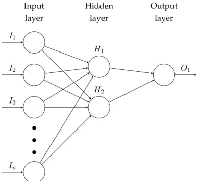
Neural networks are modelled after the manner in which the neurons in the human brain communicate and process information (Thomaset al.,2017). The multi-layer feed-forward perceptron neural network structure consists of an input layer, one or

10_{refer to (}_James_{et al.}_,₂₀₁₃_;_Han_{et al.}_,₂₀₁₁₎ 11_{discussed in more detail in section}_3.5.2

(23)

3.4 Models 14

more hidden layers and an output layer. All the independent variables are fed into the input layer. The variables are then transformed through the hidden layers and eventually a value is calculated for the output layer. At each layer, a weighted sum of the inputs is calculated for each neuron in the layer. Each neuron, in the current layer, then transforms the weighted sum through an activation function where the result will be used as an input for the next layer of the network (see figure3.2). The neural network is feed-forward and this ensures that the weights do not feed into a previous layer of the network.

An activation function is chosen by the user and for a classification problem, popular choices includethreshold, logisticortanhfunctions (Thomaset al.,2017). The number of hidden layers is user-specified.Hand and Henley(1997) argue that two hidden layers are enough for any type of prediction problem. A perceptron with no hidden layer is better suited for linearly separable data whilst a multi-layer perceptron is suited for non-linearly separable data12(Rumelhartet al.,1986).

The weights are calculated through training under back propagation algorithm with the aim of minimizing the entropy error function (Thomas et al., 2017; Han

et al.,2011;Trevoret al.,2009).

The number of neurons per hidden layer is user-specified, however, Thomas

et al.(2017) suggest that an optimal number of neurons can be determined after the initial training stage.

For binary classification, the output layer has one output value with a value that could be seen as a probability13of being classified asEmployed.

The derivation behind a neural network is difficult to interpret, however, it does have a higher tolerance to deal with noisy data and is not effected by correlation between variables unlike a logistic regression model (Hanet al.,2011).

3.4.3 Ensemble Methods

An Ensemble Method is a technique of creating a composite model. Therefore, a model based on a number of types of models (also known as base learners/classifier). Each base learner can have a sampled version of the original data set, depending on the process of the chosen ensemble method being used. A test data point is then classified into the class through a type of voting procedure.

For Homogeneous ensemble methods, we discussBagging, Boostingand Rota-tion Forests. The methodologies are similar in that they have the same type of model as a base learner but differ in the data set sampling, base classifier dependence at

12_{where it is not possible to distinguish between classes with a straight boundary line} 13_{the value is not necessarily a number between 0 and 1}

(24)

3.4 Models 15

..

.

I1 I2 I3 In H1 H2 O1 Input layer Hidden layer Output layer

Fig. 3.2:Skeleton of the multi-layer feedforward neural network model wherenis the

num-ber of variables used in the abridged data set

each iteration and weights of the voting process. For all ensemble methods we will be using decision trees as base learners for ease of interpretability14_.

For the Heterogeneous ensemble approach, we have created a model that uses an equally-weighted majority vote of the classifications given by the 5 individual classifier models discussed earlier (i.e. KNN, logistic regression, polynomialand ra-dial SVM, as well as aMulti-layer Perceptron Neural Network). This model aims to increase accuracy which could also lead to overfitting of a model on the training data.

Selective ensembles could have also been considered. These types of ensembles chose a subset of the original base models instead of using all the models.Baesens

et al.(2015) elaborate on these, however, we will not review them here.

Bagging

Bagging is a simple ensemble method that is also known as bootstrap aggregation

(Hanet al.,2011;Jameset al.,2013). For each base classifier, the original data set is resampled with replacement and therefore has repeated data points in the result-ing data set (also known as bootstrap samplresult-ing). The bootstrapped data set is fed into the base classifier algorithm to produce a model. After all base classifiers are

(25)

3.4 Models 16

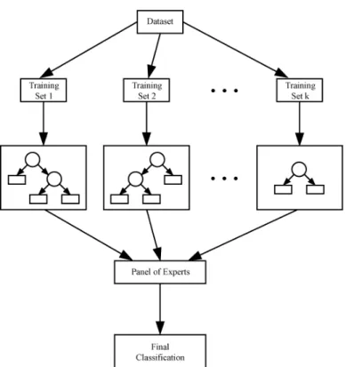
Fig. 3.3:A general view of a bagged decision tree model where each training set is a

boot-strapped version of the original data set that is fed into a decision tree base classi-fier. ThePanel of Expertsis the classification outcome of each base classifier and the

Final Classificationis a result of the majority of the classification outcomes of the base classifications

(Decision tree ensemble using Bagging algorithm,2009)

created, the test data point is fed into all the models simultaneously and a classi-fication is obtained for each base model. The data point is then classified into the class that the majority of the models have classified the data point into. Figure3.3 shows a general view of abagged decision treemodel.

The method has the advantage of reducing the variance of individual classifiers. It is also hardly affected by issues of outliers (Hanet al.,2011). Bagging, however, can suffer from bias due to dominant independent variables in the data set (James

et al.,2013), thus methods such asRandomandRotation forests(see3.4.3) were devel-oped. The method is not recommended for real time classification due to it being computationally expensive especially when there is a large number of base classi-fiers.

(26)

3.4 Models 17

Adaptive Boosting

Adaptive boostingis an ensemble method originating from the boosting method that aims to improve the performance of the algorithm (Freund and Schapire,1997). It is also known as theadaboostmethod. Boosting is different from bagging (see section 3.4.3), in that each base classifier is assigned its own vote, depending on how well it has performed as opposed to an equal vote (Hanet al.,2011).

The adaptive boosting method, introduced by Freund and Schapire (1997) focuses on improving what is considered a ”weak learner”. Thus, the method puts more emphasise on trying to improve classifiers that have a high misclassification/error rate.Freundet al.(1999) andHanet al.(2011) provide a more detailed explanation of how the algorithm works.

Adaboostdemonstrates the following advantages;

• Fast, simple and easily programmable. (Freundet al.,1999)

• it only needs the user to specify how many base learners/iterations should be constructed.

However, if the data has many outliers, the performance ofadaboostwill suffer since the method focuses on trying to improve the classification of ”difficult-to-classify” data points (Freundet al.,1999). The method also has the potential to overfit due to its focus on improving the misclassification rate and consequently will have better accuracy over abaggingmodel (Hanet al.,2011).

The base learner chosen is a decision tree with a tree depth of 1 as suggested by Antoniniet al.(2010). They state that anadaboostwith stumps handles unbalanced data sets well as the balanced error is minimised.

Rotation Forest

Rotation forestis a classifier ensemble method that is presented byRodriguezet al.

(2006). It is derived from a focus on feature extraction and can be broken down into two phases, training and classification.

In the training phase, a rotation matrix is prepared by applying Prinicipal Com-ponents Analysis (PCA)15 _{on a randomly selected subset of the original data set.} The data used needs to be completely numeric data and the categorical variables need to be transferred into dummy variables in order for the PCA to work. A clas-sification decision tree is then built on the rotated data set by applying the rotation matrix on the original data set. This decision tree is referred to as a base learner. The number of base learners is specified by the user. Each base learner will be different from the previous because of the random selection of a subset of the variables.

(27)

3.5 Performance measures 18

In the classification phase, the test data point is fed to each base learner and the average of each class prediction probability is calculated. The data point will be assigned to the class with the highest average. A more detailed derivation of this method can be found in the article byRodriguezet al.(2006).

This ensemble method follows a procedure similar to that ofbagging and ran-dom forestsin decision tree theory. Therotation forestsmethod promotes individual accuracy and diversity within the ensemble. Accuracy is achieved by retaining all principal components when creating the rotation matrix. Diversity is encouraged through the feature extraction of each base learner. The method, however, looses interpretability of variable importance once the PCA is applied to the base learner.

3.5 Performance measures

In this section, we give a simple explanation of the performance measures used in the two stages of model testing. A comparison of the performance measures is also done and is discussed in the Chapter4.

3.5.1 Confusion matrix and measures for binary classification

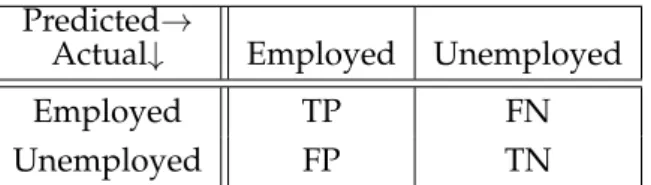
A confusion matrix is a contingency table of predicted versus actual class classifi-cation. The values in the rows represent the number of data points in the actual classification whilst the columns represent the predicted classes of the data points or vice versa. The values on the diagonal are correct classifications and all other values are misclassifications. The aim with all classification models is to reduce the number of the misclassifications. Table3.1gives the structure of the confusion matrix for the binary classification done for this dissertation. Positive classification refers to theEmployedclass and negative classification isUnemployedclass.

Numerous measures can be derived from the confusion matrix (Sokolova and Lapalme,2009). However, the measures chosen to compare the different models are based on their property of invariance as described in the article (Ballabioet al.,2018) as well as the financial cost of having a bad prediction. Therefore, we chose mea-sures that are sensitive to particular changes in the confusion matrix. It is important to see difference in measures when there is a change to a positive and negative class prediction, thereforerecallandspecificitywere selected.

Recall, also known assensitivityor as the True Positive rate (TPR), is calculated as follows, using the definitions in table3.1;

T P R= T P

(28)

It is the rate of those test data points predicted asEmployedwhen they are actually

Employed. The goal with this measure is to show the model’s ability to identify

Employeddata points. If this measure is low, i.e. approaching 0, this implies that the data points that should be identified asEmployedare being heavily misclassified and defeating the purpose of the model.

Specificity, also known as the True Negative rate (TNR), is calculated as follows, using the definitions in table3.1;

T N R= T N

T N+F P (3.2)

It can be seen as the rate of those test data points predicted asUnemployedwhen they are actuallyUnemployed. The goal with this measure is to identify the model’s ability to reject data points of other classes (Ballabioet al.,2018). The False Positive rate (FPR) can be derived from thespecificitywhere;

F P R= F P

F P +T N (3.3)

= 1−specif icity

The lower the FPR the better, as a high FPR indicates that the model is misclassi-fyingUnemployeddata points asEmployed, and this could ultimately have negative financial implications.

FPR and sensitivity are important in deriving the Receiver Operating Characteristic (ROC) curve16.

Accuracyis measure of overall effectiveness of a classifier. It is a commonly used measure for assessing classification accuracy. It is calculated, using the definitions in table3.1, as;

Accuracy = T P +T N

T P +F N +F P +T N (3.4)

The measure experiences bias against imbalanced classes and although it is usually the first to be considered it can not serve as the only measure of performance.

3.5.2 Receiver Operating Characteristic (ROC) Curves and Area under the curve (AUC)

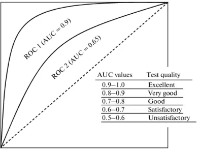
Receiver Operating Characteristic (ROC) Curve is a figure that visualises the trade-off between the True Positive rate (TPR) and the False Positive rate (FPR) along the range of all possible prediction probability thresholds that would classify the data points into classes. A good model, when analysing the ROC, will generally have a high TPR and low FPR, much likeROC1of figure3.4. This is an indication that the

(29)

Predicted→

Actual↓ Employed Unemployed

Employed TP FN

Unemployed FP TN

Tab. 3.1:Confusion matrix with a binary classification for the case of predicting

Employ-ment where TP = True Positive, FN = False Negative, FP = False Positive and TN = True Negative

positive events (i.e. predicting employment) will be predicted as positive events. If the ROC curve demonstrates a diagonal line, the TPR and FPR of positive events to negative events is the same for all prediction thresholds and the model is seen as no better than a random classifier (Hanet al.,2011). The curve can also be used to find the optimal prediction probability threshold (Thomaset al.,2017). There are a number of measures that can be calculated using the ROC curve (Ballabioet al., 2018). However, only the area under the ROC curve will be discussed here.

The area under the ROC curve (AUC) is a measure of the model’s ability to avoid false classification i.e. its discriminatory power (Sokolova and Lapalme, 2009). Therefore, the AUC measures how well is the model classifyingEmployed (Unemployed)data points asEmployed (Unemployed)predictions. A value approach-ing 1 indicates that the model is very likely to be classifyapproach-ing correctly and a value approaching 0.5 means the model has a 50/50 chance of being correct.

Sokolova and Lapalme(2009) suggest that the value of the AUC, apart from calculating the area, can be derived using information from the confusion matrix (see3.5.1) ; 1 2×( T P T P +F N + T N T N+F P) (3.5) = 1

2×(specif icity+sensitivity)

3.5.3 Gini Index

The Gini index or Gini coefficient, not to be confused with the definition used in Economics, is a measure of model performance over all possible values of the per-centage threshold that determines whether a data point is classified asEmployed

orUnemployed(Thomaset al.,2017). It is also referred to as Youden’s J Index ( Bal-labioet al.,2018;Youden,1950). It can be derived from the AUC (see 3.5.2) and is calculated as;

(30)

Fig. 3.4:General structures of Receiver Operating Characteristic (ROC) Curves

This figure demonstrates a breakdown of what the different values of the Area un-der the ROC curve could describe about the model’s overall discriminatory power

(ROC Analysis,2015)

The result is a value between 0 and 1 where 0 indicates that the model performs no better than a random classifier and 1 indicates that the model is a perfect classifier. The Gini index linearly transforms the AUC into a percentage value that calculates the performance of the classifier.

It has the disadvantage of considering all possible threshold percentage values as opposed to a selected range of threshold values.

This chapter has provided an explanation of the components in the model test-ing procedure. It started off with the data set description to provide more under-standing of the kind of data that is used. The section that follows that, is the data preprocessing section that explained how the data is transformed as well as the reasoning of why the transformation is required. There is also some elaboration of how the two-stage testing procedure is going to work with the different models and versions of the data set. A further explanation of the type of models consid-ered for testing as well as the performance measures used in evaluating the models is given. The final model parameters, for the models that require parameters, can be seen in tableB.2. In the following chapter (4) we discuss the results of the two-stage testing. It also includes some conclusions made on the data based on the data exploration that is performed.

(31)

Chapter 4 Results

This chapter is broken up into two sections. The first section is a discussion on the behaviours of the top 48 variables as per the data reduction procedure mentioned in section3.2. The second section is a review of the model performances in the two-stage testing procedure1.

Data Exploration

In stage one of the model testing process, the variables of the data set used included the top 48 variables for predictingEmployabilityaccording to the feature selection process2. The backward selection process discussed underData reductionof section 3.2is the feature selection process used. FigureB.1shows the prediction accuracy of the model against the number of variables used in the model. The model with the best overall accuracy is the one with 48 variables. TableB.1provides the question description as well as the options of the most important variables for predicting

Employability, according to the backward selection process. It is important to note that the variable names used are in the form of the original question number of the survey. This was done for the ease of reference and it would have been complicated to rename the original 178 questions.

The most dominant independent variable was the candidates employment sta-tus beingEmployed in the informal sector3, between graduating and current formal employment. The employment status of the candidate, between graduating and current employment, played a major role inEmployabilityprediction by accounting for 7 of the 48 most vital variables.

1_{Two-stage testing as explained in chapter}₃

2_{Note that the some of the 48 variables include the dummy variables that were created and there} is repetition of an original categorical variable at different category levels

3_{This means that one works for an unregistered, informal trader, maker or seller of goods and} servicesSouth Africa - Graduation Destination Survey 2012(2015)

(32)

Chapter 4. Results 23

Other noteworthy variables were whether the candidate looked for work by

responding to job advertisements through employment websites4, as well as if the can-didates primary method of finding current employment wasthrough the help of a lecturer5. Thus, the combination of the students efforts of looking for a job through online job advertisements and the assistance received from their lecturers are key features to finding employment after graduating.

It is also found that whether the candidate is studyingfull-time or part-timeis important6. One of many assumptions as to why the variable is important, could be that a part time student is more likely to get employed because they already getting work experience.

The degree level also plays an important role inEmployabilityprediction espe-cially if the degree is aMasters degree by coursework and research7.

The age range to which the candidate belonged is also important, but surpris-ingly the age range of between 22 and 30 was not important. We were more inter-ested in this age range, as it includes a lot more recent undergraduates. This could imply that this age range had such diversity between theEmployedandUnemployed

data points that it would be more difficult to predictEmployability.

TheNeighbour distance plot8_{is meant to help us identify potential clusters within} the data. The clusters are formed by firstly matching the data points to the nodes that display properties similar to that of the data point and then identify how sim-ilar the properties of the nodes are from each other by using a distance measure. The procedure of determining the number of nodes as well as the formula for di-viding the data according to certain properties is outside the scope of this disser-tation9. Heatmaps of theneighbour distanceplot as well as the individual variable plots from tableB.1are constructed using Self-Organising Maps as developed by Kohonen(1990). Looking at Figure4.1, the darker blue (red) the node is the more (dis)similar the node is to its neighbour. We would like to see two distinct clusters, where the one will represent anEmployedcluster and the other anUnemployed clus-ter. Yet, from figure4.1, we observe one oddly shaped cluster in the bottom right corner of the plot as many dark blue nodes are seen in that region. Other clusters are difficult to identify. There are a few dark red nodes which suggest significant difference to neighbours but these nodes could also be housing outliers.

4_{Question 3.1.13 Answer:f of the}_{South Africa - Graduation Destination Survey 2012}₍₂₀₁₅_{) survey} 5_{Question 3.4.6 Answer: 2 of the}_{South Africa - Graduation Destination Survey 2012}₍₂₀₁₅_{) survey} 6_{Question 2.1 Answer:1 or 2 of the}_{South Africa - Graduation Destination Survey 2012}₍₂₀₁₅_{) data} 7_{Question 2.4.1 Answer:1 of the}_{South Africa - Graduation Destination Survey 2012}₍₂₀₁₅_{) survey} 8_{also known as U-matrix}

9_{However, better elaboration and explanation of methods used are in}_Kohonen₍₁₉₉₀_);_Hua_{et al.} (2009)

(33)

Fig. 4.1:Neighbour distance plot of theSouth Africa - Graduation Destination Survey 2012

(2015) survey data

This figure shows the distance between the nodes where the darker blue (red) the node is the more (dis)similar the node is to its neighbour. An oddly shaped cluster is seen in the bottom right corner of the plot otherwise the plot seems disjoint and clusters are hard to identify

(34)

After looking at theNeighbour distance plot, we look at the individual variable

property plotsto examine which variables contribute more to certain clusters, i.e. what are the properties that cause the separation of the clusters. Thus, the aim is observe theproperty plots that behave similarly or show contrast to that of the

Neighbour distance plot. Surprisingly, theproperty plotsof the top 48 variables10 do not display patterns similar to that of theNeighbour distance plot. This discovery needs to be investigated further as it is unusual and makes it difficult to determine which variables acted as cluster dividers.

However, while observing these individual property plots we can also iden-tify which properties compliment or contrast each other. The property plot ofq2 1

andq3 3, fig4.2, behave eerily similar where the former shows information about whether the candidate did their degree part-time or full-time and the latter vari-able indicates the employment status of the candidate before pursuing their de-gree. This relationship would make sense because it is more likely that a candidate that was unemployed before pursuing their degree is more likely to be doing their degree full-time11.

Variables q3 3 and q3 3 2 seem to show inverse relationships, refer to figure 4.3. Variableq3 3seeks to identify whether the candidate worked before their 2010 qualification whilstq3 3 2indicates whether the candidate who had employment before their degree is still working at the same place after obtaining their degree. The difficulty with comparing this is thatq3 3contains the responses of those can-didates that did not work prior to the degree whilstq3 3 2does not. This could explain the distribution as possible empty nodes could be in the data. The dark red nodes in theq3 3 2plot could contain the empty nodes which corresponds to dark blue nodes in the q3 3plot that could be the responses of those candidates that were unemployed before pursuing their 2010 qualification. This way we could deduce that the candidates that were unemployed before their 2010 qualification are represented by the dark blue nodes in theq3 3plot.

10_Table_B.1

(35)

Fig. 4.2:Property plot comparison of question 2.1 and 3.3 ofSouth Africa - Graduation

Des-tination Survey 2012(2015) data

This figure shows the distance between the nodes where the darker blue (red) the node is the more (dis)similar the node’s response is to its neighbour. The property plot ofq2 1andq3 3behave eerily similar where theq2 1plot shows information distribution about whether the candidate did their degree part-time or full-time and theq3 3plot indicates the employment status of the candidate before pursuing their degree. The figures tend to have darker blue nodes at the same regions of their respective maps which shows that similar properties are seen at the data points in the nodes of these plots. We suggest that one explanation could be that a candidate that was unemployed before pursuing their degree is more likely to be doing their degree full-time. So if we assume the dark blue nodes in theq2 1

plot represent the unemployed before 2010 qualification nodes and the dark blue nodes in theq3 3plot represent the candidates doing the degree full-time*_.

(36)

Fig. 4.3:Property plot comparison of question 3.3 and 3.3.2 of South Africa - Graduation

Destination Survey 2012(2015) data

This figure shows the distance between the nodes where the darker blue (red) the node is the more (dis)similar the node’s response is to its neighbour. Variable

q3 3seeks to identify whether the candidate worked before their 2010 qualification whilstq3 3 2indicates whether the candidate who had employment before their degree is still working at the same place after obtaining their degree. The dark red nodes could contain the empty nodes which corresponds to dark blue nodes in the

q3 3plot that could be the responses of those candidates that were unemployed before pursuing their 2010 qualification.

(37)

There are individual property plots that display patterns worth noting, refer to figures4.4and4.5.

Observing the heatmap of the variableq3 4 13f, refer to figure4.4which translates to the candidatelooking for work by responding to the job ads on employment websites, the distribution is almost completely similar i.e. not much difference in the re-sponses to this variable between the nodes. This suggests that majority of the popu-lation behaved similarly in the response to this particular answer in question 3.4.13 of theSouth Africa - Graduation Destination Survey 2012(2015) data. This could im-ply that either most candidates either did or did not look for work by responding to the job ads on employment websites.

Questionq3 4 6involved identifying the primary method used by the candidate to find their current job. Figure4.5displays an interesting pattern for this question that seems to have 2 clear groupings that are not necessarily clusters because the one group is more or less dark red nodes and that implies that the nodes in that region are very different in their behaviour for that particular question, however, a very distinct cluster in the bottom right corner of the plot is observed. This clus-ter could represent the nodes that hadthrough the help of a lectureras their primary method of finding their current employment.

(38)

Fig. 4.4:Property plot of question 3.4.13 answer:f ofSouth Africa - Graduation Destination

Survey 2012(2015) data

This figure shows the distance between the nodes where the darker blue (red) the node is the more (dis)similar the node’s response is to its neighbour. The property plot of the distribution is almost completely similar (not much difference between the information contained in the nodes) suggesting that the majority of the popu-lation responded similarly to this particularly question and answer in the survey.

(39)

Fig. 4.5:Property plot of question 3.4.6 ofSouth Africa - Graduation Destination Survey 2012

(2015) data

This figure shows the distance between the nodes where the darker blue (red) the node is the more (dis)similar the node’s response is to its neighbour. The ques-tion involved identifying the primary method used by the candidate to find their current job. The property plot of the question displays an interesting pattern that seems to have 3 groupings that are not necessarily clusters. The one group is more or less dark red and that implies that the nodes in that region of very different in their behaviour for that particular question. There is also a very distinct cluster in the bottom right corner of the plot.

(40)

Model Performance Results

The best model forEmployabilityprediction is selected through a two-stage testing process. In stage one, all models discussed in section3.4are trained and tested us-ing the abridgedSouth Africa - Graduation Destination Survey 2012(2015) data set12. Table4.1summarises the performance results of stage-one testing and provides the rank of the model per performance measure as well as overall average rank of the model. The top 3 models are selected using the top 3 highest average ranks, i.e.

Adaboost, Polynomial Support Vector MachineandBagged decision trees. The parame-ters for these models can be found in tableB.2. Generally, all the models performed extremely well with the test set. Many factors could have contributed to this phe-nomenon including;

• the training and test set data set being extremely similar in nature. Similar with regards to the class imbalance of the dependent variable ( Employabil-ity) or in the data points makeup13. The class imbalance was fixed through the stratified sampling, however, the data point similarity was not tested but could possibly account for the test set doing so well.

• that the variables selected are all vital in predictingEmployabilitydespite the model used.

• that there were inclusion of too many variables to begin with and maybe more variable reduction could have taken place.

All the models had greatAccuracyandRecallwhere all of them are displaying val-ues of above 90% . A value of 100% forRecall is observed for theBagged decision treesandAdaboostmodels. Thus, these models always predicted theEmployeddata points correctly.

The Specificity did not go as well but still good nonetheless where the worst performer is theKNN14_{. This suggests that the} _KNN _{model does not predict the}

Unemployeddata points as well as the other models.

TheAdaboostmodel has the best AUC and Gini index performance values (value of 0.98361 and 0.96721 respectively). Therefore, of all the models the Adaboost15 has the best ability to avoid false classification at all possible percentage threshold values.

Theindividual classifiers16collectively performed worse overall. This should be expected given that the ensemble methods were created to improve the

perfor-12_{refer to chapter}₃_{and figure}_3.1_{for details about what is meant by the abridged data set} 13_{i.e. the data between candidates are similar}

14_k_{-Nearest Neighbour}

15_{Refer to table}_B.3_{to view the results of the variable importance of the}_Adaboost_model 16_{this is including the neural network}

(41)

mance of a individual classifiersHanet al.(2011).

(42)

Accuracy Recall Specificity AUC Gini index Average rank Logistic Regression 0.98347 (4) 0.98895 (7) 0.95082 (3) 0.96989 (7) 0.93977 (7) 5.6 k-Nearest Neigh-bours 0.92975 (9) 0.95580 (9) 0.85246 (9) 0.90413 (9) 0.80826 (9) 9 Radial SVM 0.98347 (4) 0.99448 (3) 0.95082 (3) 0.97265 (4) 0.94529 (5) 3.8 Polynomial SVM 0.98760 (2) 0.99448 (3) 0.96721 (1) 0.98084 (2) 0.96168 (2) 2 Multi-layer NN 0.96694 (8) 0.98343 (8) 0.91803 (8) 0.95073 (8) 0.90146 (8) 8 Bagged decision trees17 0.98760 (2) 1.00000 (1) 0.95082 (3) 0.97541 (3) 0.95082 (3) 2.4 Adaboost 0.99174 (1) 1.00000 (1) 0.96721 (1) 0.98361 (1) 0.96721 (1) 1 Rotation Forest 0.98347 (4) 0.99448 (3) 0.95082 (3) 0.97265 (4) 0.94529 (5) 3.8 Simple average model 0.98347 (4) 0.99448 (3) 0.95082 (3) 0.97265 (4) 0.94530 (4) 3.6

Tab. 4.1:Performance Results of the test data on the differently trained machine learning

models where SVM stands for Support Vector Machine, NN stands for Neural Network and Adaboost refers to the Adaptive Boosting model using decision trees as base classifiers. The number in parenthesis is the rank number of that model for that performance measure.

(43)

Accuracy Recall Specificity AUC Gini index Average rank Polynomial SVM 0.87597 (2) 0.93782 (2) 0.69204 (3) 0.81507 (3) 0.63013 (3) 2.6 Bagged decision trees 0.89147 (1) 0.95337 (1) 0.70769 (2) 0.83053 (2) 0.66106 (2) 1.6 Adaboost 0.87209 (3) 0.91192 (3) 0.75385 (1) 0.83288 (1) 0.66576 (1) 1.8

Tab. 4.2:Performance Results of the test data on the top 3 machine learning algorithms as

per the results in table4.1where SVM stands for Support Vector Machine and Adaboost refers to the Adaptive Boosting model using decision trees as base clas-sifiers. The number in parenthesis is the rank number of that model for that per-formance measure.

The next stage of the model testing is to remove the most important variables18 from the abridged data set at the point before the data reduction was performed on the data in the data preprocessing step19, refer to figure3.2. We now test the top 3 models with the 352 independent variables that were initially rejected by the data reduction technique. Table4.2 shows the performance results of the models using the abridged data. TheBagged decision treeshas a slight edge over theAdaboost

model. The overall performance values have indeed decreased, as expected given the new data set.

Table4.3gives a better view of the differences between the performance values of the models from the the different testing stages. At-test is performed to iden-tify whether the differences were significant, and thep-value for each performance measure is also included in table4.320.

The average difference change forSpecificityandGini indexi.e. -25% and -32% respectively, show the models seem to have become worse at correctly classifying

Unemployeddata points as well as showing a decrease in its overall ability to predict correctly regardless of probability threshold. There is also a significant change in the overallAccuracyof the models, as a result of the poor performance of predicting

Unemployeddata points . When analysing thep-value, the performance difference 18_{as per the data reduction process discussed in section}_3.2_{and resulting most important variables} displayed in TableB.1

19_{Note that the class imbalance was kept constant}

20_{More explanation of the t-test performed, the p-value as well as significance level is in section}_B.4 of the Appendix

(44)

Accuracy Recall Specificity AUC Gini

index ∆(st1, st2) ∆(st1, st2) ∆(st1, st2) ∆(st1, st2) ∆(st1, st2) Polynomial SVM -11% -6% -28% -17% -34% Bagged decision trees -10% -5% 26% -15% -30% Adaboost -12% -9% -22% -15% -31% Average Change -11% -6% -25% -16% -32% p-value 0.0342∗ 0.2307 0.045∗ 0.0144∗ 0.0144∗

Tab. 4.3:Summary of the changes in the value of the performance measures when a stress

test is performed on the top 3 machine learning models as well as the resulting p-values of thet-test performed on the differences where∗_{indicates significant at}

a 5% level of significance

can be seen as statistically significant depending on the level of significance. Look-ing at a 5% level of significance, the only measure that does not have a significant difference isSpecificity. Thus, the models still predicts the Employed data points well. This outcome supports the argument that all the variables in this data set are important to predict if one isEmployedregardless of the model used. Yet, the variables that were discarded by the data reduction technique proved to hardly contribute to predictingUnemployeddata points .

The aim of the drastic variable change is to see which model would remain re-liable when certain variables were no longer available21. The best model overall for predictingEmployabilityis theBagged decision tree. This decision is based on its consistence through both stages of testing and having the lowest difference in per-formance between the two testing stages. However, theAdaboostis a close second and it also happens to be homogeneous ensemble. Surprisingly, the heterogeneous ensemble(Simple average model)did not even pass the first round of testing. This could be because of the overall poor performance of the individual classifiers.

This chapter summarises the results of the two-stage testing process as well as 21_{The important variables are seen in table}_B.1_{in the Appendix which have a further description} of the variable.