One qubit quantum gates in a circular graphene quantum dot: genetic algorithm approach

N A N O E X P R E S S

Open Access

One-qubit quantum gates in a circular graphene

quantum dot: genetic algorithm approach

Gibrán Amparán

, Fernando Rojas

and Antonio Pérez-Garrido

Abstract

The aim of this work was to design and control, using genetic algorithm (GA) for parameter optimization, one-charge-qubit quantum logic gatesσx,σy, andσz, using two bound states as a qubit space, of circular graphene quantum dots in a homogeneous magnetic field. The method employed for the proposed gate implementation is through the quantum dynamic control of the qubit subspace with an oscillating electric field and an onsite (inside the quantum dot) gate voltage pulse with amplitude and time width modulation which introduce relative phases and transitions between states. Our results show that we can obtain values of fitness or gate fidelity close to 1, avoiding the leakage probability to higher states. The system evolution, for the gate operation, is presented with the dynamics of the probability density, as well as a visualization of the current of the pseudospin, characteristic of a graphene structure. Therefore, we conclude that is possible to use the states of the graphene quantum dot (selecting the dot size and magnetic field) to design and control the qubit subspace, with these two time-dependent interactions, to obtain the optimal parameters for a good gate fidelity using GA.

Background

Quantum computing (QC) has played an important role as a modern research topic because the quantum me-chanics phenomena (entanglement, superposition, pro-jective measurement) can be used for different purposes such as data storage, communications and data proces-sing, increasing security, and processing power.

The design of quantum logic gates (or quantum gates) is the basis for QC circuit model. There have been pro-posals and implementations of the qubit and quantum gates for several physical systems [1], where the qubit is represented as charge states using trapped ions, nuclear magnetic resonance (NMR) using the magnetic spin of ions, with light polarization as qubit or spin in solid-state nanostructures. Spin qubits in graphene nano-ribbons have been also proposed. Some obstacles are present, in every implementation, related to the proper-ties of the physical system like short coherence time in spin qubits and charge qubits or null interaction bet-ween photons, which is necessary to design two-qubit

quantum logic gates. Most of the quantum algorithms have been implemented in NMR as Shor's algorithm [2] for the factorization of numbers. Any quantum algo-rithm can be done by the combination of one-qubit uni-versal quantum logic gates like arbitrary rotations over Bloch sphere axes (X(ϕ), Y(ϕ), and Z(ϕ)) or the Pauli

gates (σx¼ 0 1

1 0

;σy¼ 0 −i

i 0

;σz¼ 1 0 0 −1

)

and two-qubit quantum gates like controlled NOT which is a genuine two-qubit quantum gate.

The implementation of gates using graphene to make quantum dots seems appropriate because this material is naturally low dimensional, and the isotope 12C (most common in nature) has no nuclear spin because the sum of spin particles in the nucleus is neutralized. This prop-erty can be helpful to increase time coherence as seen by the proposal of graphene nanoribbons (GPNs) [3] and Z-shape GPN for spin qubit [4].

In this work, we propose the implementation of three one-qubit quantum gates using the states of a circular graphene quantum dot (QD) to define the qubit. The control is made with pulse width modulation and coher-ent light which induce an oscillating electric field. The time-dependent Schrodinger equation is solved to de-scribe the amplitude of being in a QD state Cj(t). Two

bound states are chosen to be the computational basis * Correspondence:[email protected]

1

Departamento de Física Aplicada, Antiguo Hospital de la Marina, Campo Muralla del Mar, UPCT, Cartagena, 30202 Murcia, Spain

2

Departamento de Física Teórica, Centro de Nanociencias y Nanotecnologías, Universidad Nacional Autónoma de México, UNAM, Apdo, Postal 14, Ensenada, Baja California 22830, México

|0i≡|ψ1/2 |1i≡|ψ−1/2i with j= 1/2 and j=−1/2, res-pectively, which form the qubit subspace. In this work, we studied the general n-state problem with all dipolar and onsite interactions included so that the objective is to optimize the control parameters of the time-dependent physical interaction in order to minimize the probability of leaking out of the qubit subspace and achieve the de-sired one-qubit gates successfully. The control parameters are obtained using a genetic algorithm which finds effi-ciently the optimal values for the gate implementation where the genes are: the magnitude (ε0) and direction (ρ) of electric field, magnitude of gate voltage (Vg0), and pulse width (τv). The fitness is defined as the gate fidelity at the measured time to obtain the best fitness, which means the best control parameters were found to produce the de-sired quantum gate. We present our findings and the evo-lution of the charge density and pseudospin current in the quantum dot under the gate effect.

Methods

Graphene circular quantum dot

The nanostructure we used consists of a graphene layer grown over a semiconductor material which introduces a constant mass term Δ [5]. This allows us to make a confinement (made with a circular electric potential of constant radio (R)) where a homogeneous magnetic field (B) is applied perpendicular to the graphene plane in order to break the degeneracy between Dirac's pointsKandK’, distinguished by the termτ= +1 andτ=−1, respectively.

The Dirac Hamiltonian with magnetic vector field in polar coordinates is given by [6]:

H0ðr;φÞ ¼−ivσx e iφ e−iφ

∂ ∂rþvσy e

iφ e−iφ

j−

1 2

r þbr 0

0

jþ1 2

r þbr

0 B B B B B B @ 1 C C C C C C A

þτΔσxþU rð Þ;

ð1Þ

where v is the Fermi velocity (106m/s), b=eB/2, and j which is a half-odd integer is the quantum number for total angular momentum operator Jz. We need to solve

Hτψ½ j;τ ¼E½ j;τψ½ j;τ. Eigenfunctions have a pseudospinor form:

ψ½ j;τðr;φÞ ¼ei j− 1 2

ð Þφ χτAð Þr

χτ

Bð Þr eiφ

; ð2Þ

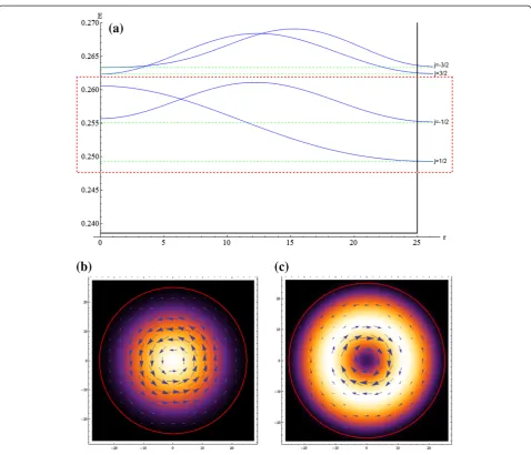
where χ are hypergeometric functions M (a,b,z) and U (a,b,z) inside or outside of radius R (see [6] for details) (Figure 1).

Due to the constant mass term and broken degene-racy, we obtain two independent Hilbert spaces. There-fore, we can choose the spaceKfor the definition of the

computational basis of the qubit to implement the quantum gates and to make the dynamic control follo-wing a genetic algorithm procedure.

The wave function in graphene can be interpreted as a pseudospinor of the sublattice of atom type A or B. In order to visualize the physics evolution due to the gate operation, we calculate the pseudospin current as the expectation values for Pauli matricesJ rð;φ;tÞ ¼j_x;j_y¼

vψðr;φ;tÞσψ ðr;φ;tÞ.

The selected states that we choose to form the compu-tational basis for the qubit are the energies (Ej): E1/2= .2492 eV andE₋1/2= .2551 eV (and the corresponding ra-dial probability distributions is shown in Figure 2a). The energy gap is E01=E−1/2−E1/2= 5.838 meV. To achieve transitions between these two states with coherent light, the wavelength required has to be λlaser¼2πc

E01¼212:35

μm, which is in the range of far-infrared lasers. Also, in controlling the magnetic fieldB, it is possible to modify this energy gap. We present as a reference point the plot for the density probability and the pseudospin current for the two-dimensional computational basis |0i= |ψ1/2 (Figure 2b) and |1i= |ψ₋1/2 (Figure 2c), where a change of direction on pseudospin current and the creation of a hole (null probability near r= 0) is induced when one goes from qubit 0 to1.

Quantum control: time-dependent potentials

First of all, we have to calculate the matrix representa-tion of the time-dependent interacrepresenta-tions in the QD basis. Then, we have to use the interaction picture to obtain the ordinary differential equation (ODE) for the time-dependent coefficient which is the probability of being in a state of the QD at time t and finally obtaining the optimal parameter for gate operation.

Electric field: oscillating These transitions can be

in-duced by a laser directed to the QD carrying a wave-length that resonates with the qubit states in order to trigger and control transitions in the qubit subspace. We introduce an electric dipole interaction [7] using a time periodic Hamiltonian with frequency ω: Vlaser(t) =eε(t)r, with parametersε(t)=ε0cosωt,ε0=ε0(cosρ, sinρ), and r=r(cosφ, sin φ), the term ρ is the direction and ε0is the magnitude of the electric field and are parameters constant in time. To determine the matrix of dipolar transitions on the basis of the QD states, the following overlap integrals must be calculated:

Vlaserljð Þ ¼t ∫

2π 0 ∫

∞

0ψ

Figure 2Diagram of genetic algorithm.Initial population of chromosomes randomly created; the fitness is determined for each chromosome; parents are selected according to their fitness and reproduced by pairs, and the product is mutated until the next generation is completed to perform the same process until stop criterion is satisfied.

the angular part defines transition rules, and as a result, we get a non-diagonal matrix; this indicates that transi-tions are only permitted between neighbor states. The matrix components are complex numbers;ε0directed in^y direction is a pure imaginary number and directed inx^is a real number.

Voltage pulse on siteThis interaction can be applied as

a gate voltage inside the QD. In order to modify the electrostatic potential, we use a square pulse of widthτv and magnitudeVg0. The Hamiltonian is

Vgateð Þ ¼t Vg0θð−tþτvþt0Þθðt−t0ÞθðR−rÞ; ð4Þ

Vgatelj¼Vg0δl;j∫ R

0χ

lð Þr χjð Þr rdr: ð5Þ

The matrix components in Equation 5 are diagonal, so this interaction only modifies the energies on the site. Since the Heaviside function θ depends on r in Equation 4, the matrix components are the probability to be inside the quantum dot which is different for each eigenstate, so this difference can introduce rela-tive phases inside the qubit subspace.

One-qubit quantum logic gates

Therefore, we have to solve the dynamics of QD prob-lem in N-dimensional states involved, where the control has to minimize the probability of leaking to states out of the qubit subspace in order to approximate the dy-namic to the ideal state to implement correctly the one-qubit gates. The total Hamiltonian for both quantum dot and time-dependent interactions is Hð Þ ¼ Ht 0þ

Vgateð Þ þt Vlaserð Þt , where H0 is the quantum dot part

(Equation 1) andVlaser(t) andVgate(t) are the time con-trol interactions given by Equations 3 and 4.

We expand the time-dependent solution in terms of the QD states (Equation 2) ψðr;φ;tÞ ¼∑

l

Clð Þt ψlðr;φÞ

as. Therefore, the equations for the evolution of prob-ability of being in state l at time t, Cl(t), in the

inter-action picture, are given by:

i∂

∂tClð Þ ¼t Vg0Vgatelθð−tþτvþt0Þθðt−t0ÞClð Þt þε0cosðωctÞ∑

jVlVlaserli;jCjð Þt e i Eð l−EjÞt:

ð6Þ

The control problem of how to produce the gates be-comes a dynamic optimization one, where we have to find the combination of the interaction parameters that produces the one-qubit gates (Pauli matrices). We solve it using a genetic algorithm [8] which allows us to avoid local maxima and converges in a short time over a

multidimensional space (four control parameters in our case). The steps in the GA approach are presented in Figure 2, where the key elements that we require to de-fine four our problem are chromosomes and fitness.

In our model, the chromosomes in GA are the array of values {Vg0, τv, ε0, ρ}, where Vg0 is the voltage pulse magnitude,τvis the voltage pulse width,ε0is the electric field magnitude, andρis the electric field direction. The fitness function, as a measure of the gate fidelity, is a real number from 0 to 1 that we define as fitness(tmed) = | <Ψobj|Ψ(tmed) > |2× | <Ψ0|Ψ(2tmed) > |2where |Ψobjiis the objective or ideal vector state, which is product of the gate operation (Pauli matrix) on the initial state |Ψ0i. Then, we evolve the dynamics to the measurement time

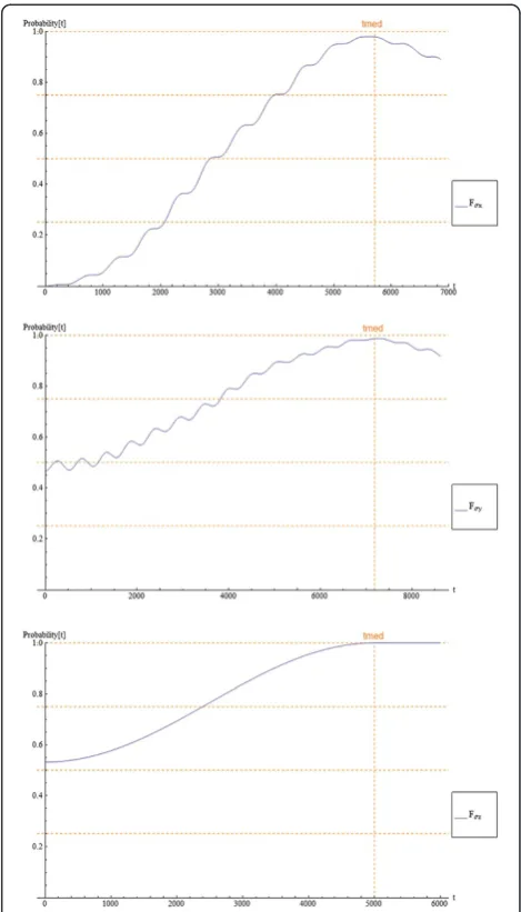
Figure 3Time evolution of gate fidelity or fitness for the three gates.Plot of gate fidelityσxin the top side,σyin the middle, and

σzin the bottom side; gate fidelity (FσIin blue where I is{x,y,z}) is the

tmed to obtain |Ψ(tmed)i. Determination of gate fidelity results in the probability to be in the objective vector state at tmed. Fitness involves gate fidelity at tmed and probability to be in the initial state at 2tmed. This gives a number between 0 and 1, indicating how effective is the transformations in taking an initial state to the objective state and back to the initial state in twice of time (the re-set phase).

The initial population of chromosomes ({Vg0,τv,ε0,ρ}) is randomly created, then fitness is determined for each chromosome (which implies to have the time-dependent evolution ofCl(t) to the measurement time); parents are

selected according to their fitness and reproduced by pairs, and the product is mutated until the next genera-tion is completed; one performs the same process until a stop criterion is satisfied.

Results and discussion

The control dynamics were done considering N= 6 states, two of them are used as the qubit basis, so that the effect of the interaction stays inside the qubit sub-space . The gate operation is completed in a time win-dow that depends on ε0, and control parameters are

defined to achieve operation inside a determined time window. The possible values of the electric field direc-tion ρ is set from 0 to 2π, pulse width τv domain is set from 0 to time window and the magnitude Vg0 is set from 0 to an arbitrary value. The genetic algorithm

procedure is executed for quantum gates σxand σy. The fitness reaches a value close to 1 near to 30 generations for both gates. The optimal parameters found for quantum gate σx are Vg0=.0003685, τv= 4215.95, ε0= .0000924, andρ= .9931π. Forσy are Vg0= .0355961, τv= 326.926, ε0= .0000735, and ρ= 1.5120π. For the quantum gate σz, genetic algorithm is not needed be-cause for this case,ε0= 0, so Equation 6 is an uncoupled

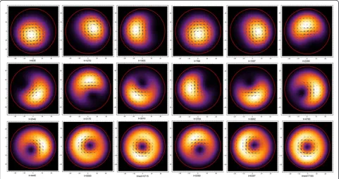
ordinary differential equation (ODE) with specific solu-tion. To achieve this gate transformation in a deter-mined time window, we can calculate Vg0, so that the control values for this quantum gate are Vg0=.1859, τv= 5,000,ε0= 0, andρ= 0.In Figure 3, we plot the time evolution of the gate fidelity or fitness for the three gates. We observe a good optimal convergence close to 1 at the time of measurement and reaching again the re-set phase. To see the state transition and the quantum gate effect in the space, it is convenient to plot the dens-ity probabildens-ity in the quantum dot and the correspond-ing pseudospin current, where we see how the wave packet has different time trajectory according to the gate transformation. For instance, the direction and time of creation of the characteristic hole (null probability) in the middle of the qubit one, which correspond more or less to an equal superposition of the qubit zero and one (column 2 and row 2 in Figure 4, right). This process has to be different for σy because it introduces an im-aginary phase in the evolution which is similar with the

Figure 4Time evolution of probability density and pseudospin current for the quantum gateσxandσyoperation.Time evolution of

density and current probability due to the effect of the produced quantum gateσxin the left side andσyin the right side, initial state |Ψ0i= |0i

change of the arrow directions in the pseudospin current. The same situation arises for σz (result not shown), but in this case, we use as an initial state

Ψ0i ¼ 1ffiffi 2

p _{ðj0i þj Þ1i}

, which is similar to the plot of

col-umn 2 and row 2 in Figure 4 (left) and then to show ex-plicitly the gate effect of introducing the minus in the one state to reach a rotated state similar to plot of col-umn 2 and row 2 in Figure 4 (right).

Conclusions

We show that with a proper selection of time-dependent interactions, one is able to control or induce that leakage probability out of the qubit subspace in a graphene QD to be small. We have been able to optimize the control parameters (electric field and gate voltage) with a GA in order to keep the electron inside the qubit subspace and produce successfully the three one-qubit gates. In our results, we appreciate that with the genetic algorithm, one can achieve good fidelity and found that little vol-tage pulses are required for σx and σy and improve gate fidelity, therefore making our proposal of the graphene QD model for quantum gate implementation viable. Fi-nally, in terms of physical process, the visualization of the effects of quantum gatesσxandσyis very useful, and clearly, both achieve the ideal states. The difference bet-ween them (Figure 4) is appreciated in the different tra-jectories made by the wave packet and pseudospin current during evolution due to the introduction of rela-tive phase made by gateσy.

Competing interests

The authors declare that they have no competing interests.

Authors_’contributions

The work presented here was carried out collaboration among all authors. FR and APG defined the research problem. GA carried out the calculations under FR and APG's supervision. All of them discussed the results and wrote the manuscript. All authors read and approved the final manuscript.

Acknowledgments

The authors would like to thank DGAPA and project PAPPIT IN112012 for financial support and sabbatical scholarship for FR and to Conacyt for the scholarship granted to GA.

Received: 15 November 2012 Accepted: 18 April 2013 Published: 16 May 2013

References

1. Ladd TD, Jelezko F, Laflamme R, Nakamura Y, Monroe C, O’Brien JL: Quantum computers (review).Nature2010,464:45–53.

2. Vandersypen LM, Steffen M, Breyta G, Yannoni CS, Sherwood MH, Chuang IL:Experimental realization of Shor's quantum factoring algorithm using nuclear magnetic resonance.Nature2001,414:883–887.

3. Trauzettel B, Bulaev DV, Loss D, Burkard G:Spin qubits in graphene quantum dots.Nature Physics2007,3:192–196.

4. Guo G-P, Lin Z-R, Tao T, Cao G, Li X-P, Guo G-C:Quantum computation with graphene nanoribbon.New Journal of Physics2009,11:123005. 5. Zhou SY, Gweon G-H,et al:Substrate-induced band gap opening in

epitaxial graphene.Nature Materials2007,6:770–775.

6. Recher P, Nilsson J, Burkard G, Trauzettel B:Bound states and magnetic field induced valley splitting in gate-tunable graphene quantum dots. Physical Review B2009,79:085407.

7. Fox M:Optical Properties of Solids.InQuantum Theory of radiative absorption and emission Appendix B.Oxford: Oxford University Press; 2001:266–270.

8. Chong EKP, Zak SH:An introduction to optimization.InChapter 14: Genetic Algorithms.2nd edition. Weinheim: Editorial WILEY; 2001.

doi:10.1186/1556-276X-8-242

Cite this article as:Amparánet al.:One-qubit quantum gates in a circular graphene quantum dot: genetic algorithm approach.Nanoscale Research Letters20138:242.

Submit your manuscript to a

journal and benefi t from:

7 Convenient online submission

7 Rigorous peer review

7 Immediate publication on acceptance

7 Open access: articles freely available online 7 High visibility within the fi eld

7 Retaining the copyright to your article