Hidden panel cointegration

Munich Personal RePEc Archive

Hidden panel cointegration

Abdulnasser, Hatemi-J

UAE University

June 2011

Hidden Panel Cointegration

Abdulnasser Hatemi-J

UAE University

E-mail: [email protected]

Abstract

This article extends the seminal work of Granger and Yoo (2002) on hidden cointegration

to panel data analysis. It shows how cumulative negative and positive changes can be

constructed for each panel variable. It also shows how tests similar to the augmented

Dickey-Fuller tests can be implemented to find out whether the cointegration is hidden in

the panel or not. An application is provided to investigate the impact of permanent

positive and negative shocks in the government expenditure on the national output in a

panel of three countries.

Running Title: Hidden Panel Cointegration

JEL Classification: C33, H21

Keywords: Asymmetry, Panel Data, Cointegration, Testing, Government Spending,

Output

1. Introduction

Since the pioneer work of Granger (1981) cointegration analysis has become an integral

part of applied econometrics when the underlying variables are measured across time.

Based on Granger’s definition, cointegration occurs in a situation in which a linear combination between integrated variables has one unit root less than the integration order

of the variables in the model. The variables cointegrate if and only if they have common

stochastic trends that cancel each other out. There is a massive literature on cointegration

indicating its due importance. Cointegration analysis is important in empirical research in

order to avoid spurious results based on a regression model. It is also important for

analyzing the long-run relationships between the underlying variables combined with the

Testing for cointegration was initiated by Engle and Granger (1987) via implementing

residual based tests for cointegration. More robust tests where suggested by Phillips

(1987) as well as Phillips and Ouliaris (1990). Multivariate tests for cointegration were

developed by Johansen (1988, 1991), Johansen and Juselius (1990) as well as Stock and

Watson (1988). The idea to conduct tests for unit roots within a panel system originates

from Quah (1994). Tests for panel cointegration were suggested by Pedroni (1999, 2004),

Kao (1999) and Westerlund (2007), among others.

In all previous literature on cointegration testing, there was no separation between the

impact of negative and positive shocks until Granger and Yoo (2002) introduced the

concept of hidden cointegration for time series data. It is hidden in the sense that there

might not be cointegration between the variables in the original format but when the

impact of positive shocks is separated from the impact of negative shocks then

cointegration might exist between the components of the variables. The aim of this article

is to extend the concept of hidden cointegration to panel data analysis. The suggested

tests in this paper are applied to investigate the impact of contractionary as well as

expansionary fiscal policy on the economic performance in a panel consisting of

Denmark, Norway and Sweden.

The article continues as the following. Section 2 introduces hidden panel cointegration

analysis. Section 3 provides an application. The last section concludes the article. Finally,

an appendix at the end of the article provides a simple mathematical example that shows

the necessary condition for cointegration in a panel system.

2. Hidden Panel Cointegration

Consider the following variables that are integrated of the first degree, with the

resultant solution for each that is found by the recursive approach:1

∑

1

∑

For i=1, …, m. Where m signifies the cross-sectional dimension (which is two in this

particular case) and e is the disturbance term that is assumed to be a white noise process.

The positive and negative shocks for each panel variable are defined as

( ), ( ), ( ) and ( ).

Using these results, the following can be obtained:

∑

∑

∑

∑

Assume that our dependent variable is y, and then the two potential panel cointegration

equations for the components can be defined as

(1)

(2)

The positive cumulative shocks are cointegrated in the panel if is stationary.

Likewise, the negative cumulative shocks are cointegrated in the panel if is

stationary.2

2

It should be mentioned that other combinations are also possible. Such as, cumulative positive changes of

There is potentially a battery of the tests available in the literature that can be used

for testing whether as well as is stationary or not. However, the well-known

augmented Dickey-Fuller (ADF) test is the simplest one that can be used for this purpose.

Assume that we wish to test for cointegration in the panel model (1). Then, the panel

ADF test equation is the following:

∑

The optimal lag order l can be determined by minimizing an information criterion. The

null hypothesis of no cointegration between the positive components is . It is also

possible to allow for deterministic components such as individual drifts and trends in

equation (3) if necessary. Based on the results provided by Kao (1999), the following test

statistics can be used to test the null hypothesis of no panel cointegration:

√

√

Where is the t-statistic for parameter in equation (3). The variance is estimated as

, and the long-run variance is estimated as

.

Let [

]

. The variance-covariance for is estimated as

[

] _{∑ ∑}

The long-run variance-covariance matrix is estimated via the kernel estimation approach

[

]

∑ [ ∑

∑

∑

]

Where is representing the kernel function and b is the bandwidth.

The ADF test as presented in equation (4) has a standard normal distribution

asymptotically. For a proof see Kao (1999). To test for stationarity in the linear

combination between negative components as presented in equation (2), a similar ADF

test can be conducted. Other combinations are also possible.3 A Gauss code for constructing cumulative sums of positive and negative changes of each variable for each

cross sectional unit in the panel is available on request from the author.4

3. An Application

The suggested test for hidden panel cointegration is applied to investigating the long-run

relationship between government spending and economic performance in Denmark,

Norway and Sweden. Quarterly data is used during the period 1993-2010. The source of

the data is the statistical bureau of each country. In order to capture real effects, the

variables are expressed at constant prices. The cumulative sums of positive and negative

shocks were constructed based on the procedure presented in the previous section. Prior

to testing for panel cointegration, panel unit root tests were implemented by using the Im,

Pesaran and Shin (2003) test. The results are presented in Table 1, which show that each

panel variable has one unit root.

3

It should be mentioned that it is also possible to test for hidden panel cointegration using other tests such as seven residual based testes suggested by Pedroni (1999, 2004) as well as panel version of the multivariate Johansen (1991) test as developed by Maddala and Wu (1999) based on the Fisher (1932) principle of deriving a combined test using the individual test results.

4

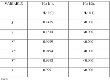
Table 1: The Results of Panel Unit Root Tests.

VARIABLE H0: I(1),

H1: I(0)

H0: I(2),

H1: I(1)

0.1485 <0.0001

0.1314 <0.0001

0.9999 <0.0001

0.9494 <0.0001

0.9998 <0.0001

0.9991 <0.0001

Notes

The denotation S stands for the log of government spending and Y is representing the log of GNP.

The Im, Pesaran and Shin (2003) test is used to test for panel unit root. P-values are presented.

Given that each variable in the panel has one unit root, it is crucial to conduct tests for

panel cointegration. The results of these tests based on equation (4) are presented in

Table 2, which indicate that there is no cointegration between government spending and

output in the panel sample for these three countries. Tests for cointegration between

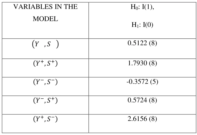
Table 2: The Results of Panel Cointegration Tests.

VARIABLES IN THE

MODEL

H0: I(1),

H1: I(0)

( ) 0.5122 (8)

1.7930 (8)

-0.3572 (5)

0.5724 (8)

2.6156 (8)

Notes

The values in the parenthesis indicate the bandwidth in the kernel estimation. The null hypothesis of no

panel cointegration is rejected at the 5% significance level if the estimated test value is lower than -1.64.

4. Conclusions

The aim of this article is to extend the hidden cointegration tests of time series data as

developed by Granger and Yoo (2002) to hidden cointegration tests of panel data. It is

shown how cumulative sums of positive and negative changes can be constructed. An

augmented Dickey-Fuller test for a panel system can be implemented to test the null

hypothesis of no panel cointegration between different components of the underlying

variables. A user friendly Gauss algorithm is produced to transform the panel variables

into their respective components.

The suggested test procedure is applied to investigating the impact of government

spending on economic output in a panel of three countries—namely Denmark, Norway

and Sweden. The results show that there is no panel cointegration between these variables

or their components. This surprising finding of no panel cointegration between GNP and

government spending in Denmark, Norway and Sweden might provide empirical support

for the existence of the Ricardo equivalence theorem in these countries. According to this

the government expenditure now means an equivalent increase in the taxes in the future.

Hence, they will adjust their behavior in such a way that there will be no real effects of

increases in the government expenditure on the economy.

In this particular case, the same cointegrational inference was obtained in the panel

regardless if the impact of positive shocks is separated from the impact of negative

shocks or not. This might be indicative of the strength of the empirical findings.

Nevertheless, future applications of the test might indicate cases in which the panel

cointegration is indeed hidden. In addition, separating the impact of positive shocks from

the negative ones might be informative per se, in order to capture the potential

asymmetry that might prevail.

References

Engle, R. F., and Granger, C. W. J. (1987) Co-integration and Error Correction:

Representation, Estimation and Testing, Econometrica, 55(2), 251-276.

Fisher, R.A. (1932) Statistical Methods for Research Workers, Oliver & Boyd,

Edinburgh, 12th Edition.

Granger, C. (1981) Some Properties of Time Series Data and Their Use in

Econometric Model Specification, Journal of Econometrics, 16, 121-130.

Granger, C.W., and Yoon, G. (2002) Hidden Cointegration. Department of Economics

Working Paper. University of California. San Diego.

Hatemi-J A. (2010) Asymmetric Causality Tests with an Application, Empirical

Economics, forthcoming.

Hatemi-J A. (2011a) Asymmetric Panel Causality Tests with an Application,

Unpublished Manuscript.

Hatemi-J A. (2011b) Asymmetric Generalized Impulse Response Functions and

Variance Decompositions, Unpublished Manuscript.

Im, K. S., Pesaran, M. H. and Shin, Y. (2003) Testing for Unit Roots in

Heterogeneous Panels, Journal of Econometrics, vol. 115(1), 53-74.

Johansen, S. (1988) Statistical Analysis of Cointegration Vectors, Journal of

Johansen, S. (1991) Cointegration and Hypothesis Testing of Cointegration Vectors in

Gaussian Vector Autoregressive Models, Econometrica, Vol.59, No.6, 1551–1580.

Johansen S. and Juselius, K., (1990) Maximum Likelihood Estimation and Inference

on Cointegration–with Applications to the Demand for Money, Oxford Bulletin of

Economics and Statistics, Vol. 52, No. 2, 169–210.

Maddala, G. S., and Wu, S. (1999) A Comparative Study of Unit Root Tests with

Panel Data and New Simple Test, Oxford Bulletin of Economics and Statistics, 61,

631-652.

Quah, D. (1994) Exploiting Cross Section Variation for Unit root Inference in

Dynamic Data. Economics Letters, 44, 9-19.

Pedroni, P. (1999) Critical Values for Cointegration Tests in Heterogeneous Panels

with Multiple Regressors, Oxford Bulletin of Economics and Statistics, 61, 653-670.

Pedroni, P. (2004) Panel Cointegration, Asymptotic and Finite Sample Properties of

Pooled Time Series tests with an Application to the PPP Hypothesis, Econometric

Theory, 20, 597-625.

Phillips, P.C.B. (1987) Time Series Regression with a Unit Root, Econometrica 55,

277-301.

Phillips, P.C.B, and Ouliaris S. (1990) Asymptotic Properties of Residual Based Tests

for Cointegration, Econometrica 58, 165-193

Stock, J. and Watson M. (1988) Testing for common trends, Journal of the American

Statistical Association, 83, 1097–1107.

Westerlund J. (2007) Testing for Error Correction in Panel Data. Oxford Bulletin of

Appendix

An Example regarding Panel Cointegration

Let us be more explicit about panel cointegration between two integrated variables by

a simple example. Consider the following two non-stationary panel variables:

(A1)

(A2)

Where and are two white noise error terms. Assuming that the initial values are

zero, continuous substitutions give the following solutions:

∑

∑

By taking the first difference of each variable, we obtain

∑ ∑

∑ (∑

)

(A6)

That is, each variable becomes stationary after taking the first difference. Hence, the

variables are integrated of the first order, denoted I(1). Now the question is if these two

panel variables are cointegrated. Denote Yt as the difference between the two variables,

∑ (∑

)

This difference is clearly a stationary process. That is, a linear combination of the

non-stationary variables is non-stationary in the panel, which in turn means that the variables

cointegrate with (1.0, -1.0) as cointegrating vector. It should be noted that the variables

cointegrate because their stochastic trend cancels each other out. In another word, the

variables have a common stochastic trend. This is the case in the hidden panel

cointegration analysis also. In order to have hidden panel cointegration, there must be at

least one common stochastic trend between the cumulative components of the positive or