A social discount rate for Turkey

Munich Personal RePEc Archive

A social discount rate for Turkey

Halicioglu, Ferda and Karatas, Cevat

Department of Economics, Yeditepe University

2011

A Social Discount Rate for Turkey

Abstract

Social Discount Rate (SDR) is a very crucial policy parameter in public project

appraisals due to its resource allocation impacts. This study estimates an SDR for

Turkey using the Social Time Preference Rate (STPR) approach. The elasticity of the

marginal utility consumption, which is the most important component of the STPR,

is estimated econometrically from a demand for food approach during the period of

1980-2008. The overall result indicates that the SDR for Turkey is 5.06%. The

European Union requires evaluation of the publicly supported commercial projects in

terms of the SDR; hence the findings from this study can be used as a useful policy

measurement for a full EU member candidate country, Turkey.

Keywords: social discount rate; social time preference; project appraisal; ARDL;

Turkey.

JEL Classifications: H20; C22.

Correspondance:

Ferda HALICIOGLU Cevat KARATAS

Corresponding author Co-author

Department of Economics Department of Economics

Yeditepe University Yeditepe University

Istanbul 34755 Istanbul 34755

Turkey Turkey

1 Introduction

Public projects and regulations have impacts that occur over time. For instance,

infrastructure projects, such as motorways, bridges or dams, have effects that occur

over decades. The Social Discount Rate (SDR) measures the rate at which a society

is willing to trade present for future consumption. Thus, the SDR is a very crucial

parameter in public project appraisals as it could considerably alter the resource

allocation and efficiency. If this rate is too high, future generations will face excess

financial burden since distant cash flows will become negligible. If this rate is too

low, ineffective projects are chosen creating an inefficient allocation of resources.

There is a consensus amongst the public policy makers that future impacts should be

discounted at the SDR. At this rate, society discounts future costs and benefit and

converts them into present values. There is, however, less agreement over what this

rate should be and how to determine it.

The existing literature on the SDR suggests that there are three main methods that are

utilized to measure the value: i) Social Time Preference Rate (STPR) approach

which is based on classical Ramsey (1928) model of saving and growth. A number

of studies such as Kula (1984 and 2004), Evans and Sezer (2002), Evans (2005), and

Percoco (2008) have adopted this approach;ii) Specifying a benchmark financial rate

approach which is based on the long-term treasury interest rates. This method is

adopted by the US Office of Management and Budget. The financial discount rate for

30 year projects is 2.8% based on 1979-2008 average. Florio (2006) provides a

fruitful discussion on this approach; iii) Trade-offs in financial markets approach

which measures the SDR as the opportunity cost of private investment instead of

According to Spackman (2004), the STPR is an appropriate measure of the SDR. The

primary concern of this paper is to estimate Turkey’s social discount rate for

long-term social projects using the demand for food approach of the STPR. As far as this

paper is concerned, no previous study has been carried out to estimate the SDR based

on the STPR for Turkey using the demand for food approach. Therefore we aim to

fill this gap in the literature. Regarding this fact the European Union requires

evaluation of the publicly supported commercial projects in terms of the SDR; hence

the findings from this study can be used as a useful policy measurement for a full EU

member candidate country, Turkey.

2 Explanation of the STPR components

Marglin (1963) and Feldstein (1965) provide the theoretical derivation of the STPR

formula which is expressed as follows:

1 ) / 1 ( ) 1

(  

 e 

g

STPR (1)

whereg is the growth rate of per capita real consumption (income),e is the absolute

value of the elasticity of the marginal utility of consumption (income), and π is the

average probability of survival of an individual: a measuer that may be used for pure

time discount rate.

Elasticity of the marginal utility of consumption (e)

For the purpose of estimating appropriate SDR, the measurement of e plays a crucial

various approaches to the measurement of e and the problems involved. There are

basically two most common approaches to estimate it: a) the personal taxation

model, which elicits the value ofe by observing the structure of the personal income

tax (Stern, 1977). Spackman (2006) argues that this approach has serious limitations.

Therefore, estimates will be biased downwards; b) demand for food models which is

proposed by Fellner (1967) assuming thate is a function of consumer preferences as

revealed by the demand for food since food is deemed to be a preference independent

good.

In this study, estimates of e are derived similar to the study of Kula (1984).

According to Kula (1984), e is measured by the ratio of income elasticity to

compensated price elasticity of the food demand function; expressed as follows:

2 1/eˆ

e

e (2)

where e₁ is income elasticity of the food demand function and eˆ₂ is the compensated

price elasticity that is obtained by eliminating the income effect from the

uncompensated price elasticity, e₂.

In order to estimate income and price elasticities, the following econometric food

demand equation is formed for Turkey in natural logarithm as follows:

t t t

t a e y e p q

where, a is the constant term, f is the per capita real consumption of food

expenditures, y is the per capita real income, p and q are price indices for food and

non-food, respectively, ε is the stochastic error term, andt is the time subscript.

The compensated price elasticity is obtained as follows:

)) ( (

ˆ₂ e₂ e₁

e    (4)

where (α) is the share of food in a consumer’s budget. Eq.(4) also refers to the

standard Slutsky equation for the relation of compensated responses to price changes

written in elasticity form. As we calculate the value of eˆ₂, e₂ is considered in

absolute value too.

Growth of per capita real consumption (g)

This parameter is usually proxied by average performance of over past time series

data; see for example, Evans (2004) and Evans and Sezer (2005). Some researchers

also use the growth rate of the economy as a substitute measurement; see for

example, Percoco (2008). In this study, we will adopt the first approach.

Calculation of the mortality based pure time discount rate (π)

The estimation of appropriate value of the pure time preference is a long-standing

debate in the economics literature, since choosing a value for this parameter requires

studies on this issue rely on different values for it. Some researchers derive it from

the individual risk of death (e.g. Kula 2004 and Lopez 2008).

This approach assumes that each member of a country discounts their future by the

probability of not being alive over a period of time. Therefore, for example, a

two-period analysis of average death rate in a country will provide the annual average

survival probability for a typical person. Thus, a similar approach is adopted in this

study.

3 Estimations and Results

Recent advances in econometric literature dictate that the long-run relation in Eq.(3)

should incorporate the short-run dynamic adjustment process. It is possible to

achieve this aim by expressing Eq.(3) in an error-correction model (ECM) as

suggested by Engle-Granger (1987). Then, the equation becomes as follows:

t t m

i

m

i

m

i

i t i

t i

t

t b b f b y b p q

f         

 _

  

 









1

1

2

0

3

0 3 2

1

0 ( / ) (5)

where  represents change,  is the speed of adjustment parameter and _t1 is the

one period lagged error correction term, which is estimated from the residuals of Eq.

(3). The Engle-Granger method requires that all variables in Eq.(5) are integrated of

order one, I(1) and the error term is integrated order of zero, I(0) for establishing a

cointegration relationship. If some variables in Eq.(3) are non-stationary, we may use

a new cointegration method proposed by Pesaran et al. (2001). This approach is also

(1987) two steps into one by replacing t₁ in Eq.(5) with its equivalent from Eq.(3).

1



t

 is substituted by linear combination of the lagged variables as in Eq.(6):

t t t t n i n i n i i t i t i t i

t c c f c y c p q c f c y c p q v

f           

 _{  }

  

 









1 1 2 0 3 0 3 2 1

0 ( / ) ( / ) (6)

The bounds testing procedure is based on a Wald (W) or Fischer (F) type statistics

and this is the first step of the ARDL cointegration method. Accordingly, a joint

significance test that implies no cointegration under the null hypothesis, (H0:

0

6 5 4 c c 

c ), against the alternative hypothesis, (H1: at least one of c4 to c6 0)

should be performed for Eq. (6). The critical values that are tabulated of an upper

bound on the assumption that all variables are I(1) and a lower bound on the

assumption that all variables are I(0). For cointegration, the calculated F or W

statistics must be greater than the upper bound.

Once a long-run relationship has been established, Eq.(6) is estimated using an

appropriate lag selection criterion. At the second step of the ARDL cointegration

procedure, it is also possible to obtain the ARDL representation of the error

correction model. To estimate the speed with which the dependent variable adjusts to

independent variables within the bounds testing approach, following Pesaran et al.

(2001) the lagged level variables in Eq.(6) are replaced by ECt-1 as in Eq.(7):

t t k i k i k i i t i t i t

t d y p q EC

f           

 _

  

 









1 1 2 0 3 0 3 , 2 1

0 ( / ) (7)

between the variables. Pesaran et al. (2001) cointegration approach has some

methodological advantages in comparison to other single cointegration procedures.

Reasons for the ARDL are: i) endogeneity problems and inability to test hypotheses

on the estimated coefficients in the long-run associated with the Engle-Granger

(1987) method are avoided; ii) the long and short-run coefficients of the model in

question are estimated simultaneously; iii) the ARDL approach to testing for the

existence of a long-run relationship between the variables in levels is applicable

irrespective of whether the underlying regressors are purely stationary I(0), purely

non-stationary I(1), or mutually cointegrated; iv) the small sample properties of the

bounds testing approach are far superior to that of multivariate cointegration, as

argued in Narayan (2005).

Time series data between 1980 and 2008 is used to estimate Eq.(3) with the ARDL

procedure. Data is collected from House Hold Budget Surveys of Turkish Institute of

Statistics (www.turkstat.gov.tr), European Marketing Data and Statistics

(www.euromonitor.com), and Istanbul Chamber of Commerce (www.ito.org.tr).

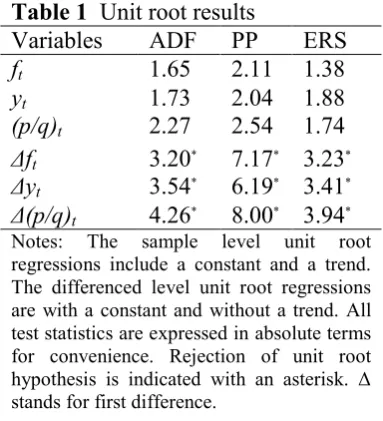
Three tests were used to test unit roots in the variables: Augmented Dickey-Fuller

(1981), Phillips-Perron (1988), and Elliott-Rothenberg-Stock (1996). Unit root tests

results are displayed in Table 1 warrant for applying the ARDL approach to

cointegration since all variables included in the model are I(1). Visual inspections of

Table 1 Unit root results

Variables ADF PP ERS

ft 1.65 2.11 1.38 yt 1.73 2.04 1.88 (p/q)t 2.27 2.54 1.74 Δft 3.20* 7.17* 3.23* Δyt 3.54* 6.19* 3.41* Δ(p/q)t 4.26* 8.00* 3.94*

Notes: The sample level unit root regressions include a constant and a trend. The differenced level unit root regressions are with a constant and without a trend. All test statistics are expressed in absolute terms for convenience. Rejection of unit root hypothesis is indicated with an asterisk. Δ stands for first difference.

Table 2 displays the cointegration tests. According to Table 2, there exists a long-run

relationship amongst the variables of Eq.(3).

Table 2The results of F and W tests for cointegration

The assumed long-run relationship; (f y,(p/q))

F-statistic 95% LB 95% UB 90% LB 90% UB

8.85 4.24 5.40 3.44 4.46

W-statistic

26.57 12.73 16.20 10.32 13.38

If the test statistic lies between the bounds, the test is inconclusive. If it is above the upper bound (UB), the null hypothesis of no level effect is rejected. If it is the below the lower bound (LB), the null hypothesis of no level effect cannot be rejected.

The summary ARDL results with some diagnostic tests are presented in Table 3. The

overall empirical results appear to be rather satisfactory. The lag selection procure

Table 3 ARDL cointegration results

Panel A. Estimated long-run coefficients: ARDL (1,3,3) selected based on the Akaike Information Criterion.

Dependent variable f_t

Regressor Coefficient Standard error T-ratio

t

y 0.870* _{0.175 4.964}

t

q p/ )

( -0.727* _{0.110 6.563}

Constant -0.927*** _{0.499 1.857}

Panel B. Error-correction representation results.

Dependent variablef_t

Regressor Coefficient Standard error T-ratio

t

y

 0.823* _{0.161 5.111}

1



 t

y 0.311** _{0.173 1.798}

2



 t

y -0.298*** _{0.177 1.677}

t

q p/ ) (

 -0.035 0.110 0.318

1 ) / (   t q

p 0.161*** _{0.085 1.880}

2 ) / (   t q

p 0.220* _{0.085 2.590}

1



t

EC -0.623* _{0.127 4.884}

Diagnostic tests

2

R 0.75 F-statistic 13.7* _SC2 (1) 2.01 _FF2 (1) 0.24

RSS 0.03 DW-statistic 2.39 2₍₂₎

N

 0.34 H2(1) 0.06

*

, **, and,*** indicate, 1%, 5%, and 10% significance levels respectively. RSS stands for residual sum of squares. T-ratios are in absolute values._SC2 , 2_FF, 2_N, and _H2 are Lagrange multiplier statistics for tests of residual correlation, functional form mis-specification, non-normal errors and heteroskedasticity, respectively. These statistics are distributed as Chi-squared variates with degrees of freedom in parentheses. The critical values for

84 . 3 ) 1 ( 2 _

 and 2(2)5.99 are at 5% significance level.

On the basis of the coefficients obtained from Panel A of Table 3 and with a budget

share of food in Turkey 24.5% during the estimation period, Eq.(4) reveals that

516 . 0 ) 830 . 0 )( 245 . 0 ( 727 . 0

ˆ₂   

e

As we substitute eˆ₂ in Eq.(2) along with the absolute estimate value of e₁, we

compute the value of e as follows:

686 . 1 516 . 0 / 870 . 0   e

The average growth rate of per capita real consumption for the period of 1980-2008

death rate is 6.1 per 1000 or 0.61% during 1980-2008. Therefore, survival

probabibility of a person is computed as  10.00610.9939, which is also

considered to represent the mortatility based time discount rate in Turkey.

Subsituting all the estimates of component parameters of the STPR in Eq.(1), we

obtain the following result for Turkey:

0506 . 0 1 ) 9939 . 0 / 1 ( ) 026 . 0 1

(  1.686  



STPR or 5.06%.

4 Concluding Remarks

This study reveals that the SDR for Turkey based on the STPR is 5.06% and it is

appropriate for application in social project appraisals. This rate is very close to the

5% discount rate proposed by the European Commission (2002) but it is not based on

any empirical analysis. Considering Turkey is on the way to become a full member

of the EU, this paper recommends application of 5.06% for different investment

decisions in the public sector of Turkey. We also draw attention to the fact that we

suggest this rate because it is very close to other empirical estimates derived for

developing countries and there exists no other STPR as being estimated for Turkey

as far as this research is concerned.

Acknowledgement

The authors would like to thank Professor Erhun Kula of Bahcesehir University for

providing insightful and valuable comments on an earlier draft of this paper. The

References

Azar, A. S. (2007) Measuring the US social discount rate. Applied Financial

Economics Letters,3, 363-66.

Cowell, F. A. and Gardiner, K. (1999) Welfare weights (STICERD). Research

Paper, No.20, London School of Economics.

Dickey D. A. and Fuller, W. A. (1981) Likelihood ratio statistics for autoregressive

time series with a unit root.Econometrica,49, 1057–1072.

Elliott, G., Rothenberg, T., and Stock, J. (1996) Efficient tests for an autoregressive

unit root. Econometrica,64, 813–836.

Engle, R. F. and Granger, C. W. (1987) Cointegration and error correction:

representation, estimation and testing.Econometrica,55, 251–276.

European Commission (2002)Guide to Cost-Benefit Analysis of Investment Projects,

DG Regional Policy.

Evans, D. J. (2005) The elasticity of marginal utility of consumption: estimates for

20 OECD countries.Fiscal Studies,26, 197-224.

Evans, D. J. (2004) A social discount rate for France.Applied Economics Letters,11,

803-808.

Evans, D. J. and Sezer, H. (2005) Social discount rates for member countries of the

European Union.Journal of Economic Studies,32, 47-59.

Evans, D. J. and Sezer, H. (2002) A time preference measure of the social discount

rate for the UK.Applied Economics,34, 1925-1934.

Feldstein, M. S. (1965) Opportunity cost calculations in cost-benefit analysis.

Fellner, W. (1967) Operational utility; the theoretical background and measurement,

in Ten Economic Studies in the Tradition of Irving Fisher (Ed.) W. Fellner, John

Wiley, New York.

Florio, M. (2006) Cost-benefit analysis and European Union cohesion fund: on the

social cost of capital and labour.Regional Studies,40, 211-240.

Kula, E. (2004) Estimation of a social rate of interest for India. Journal of

Agricultural Economics,55, 91-99.

Kula, E. (1984) Derivation of social time preference rates for the US and Canada.

The Quarterly Journal of Economics,99, 873-882.

Lopez, H. (2008) The social discount rate: estimates for nine Latin American

countries.Policy Research Papers, No.4639, The World Bank.

Marglin, S. A. (1963) The opportunity cost of public investment. The Quarterly

Journal of Economics,77, 95-111.

Narayan, P.K. (2005). The saving and investment nexus for China: evidence from

cointegration tests.Applied Economics,37, 1979–1990.

Percoco, M. (2008) A social discount rate for Italy. Applied Economics Letters,15,

73-77.

Pesaran, M. H., Shin, Y. and Smith, R. (2001) Bounds testing approach to the

analysis of level relationships.Journal of Applied Econometrics,16, 289–326.

Phillips, P. C. B. and Perron, P. (1988) Testing for a unit root in time series

regression.Biometrika,75, 335–346.

Ramsey, F. P. (1928) A mathematical model of theory of saving. Economic Journal,

Spackman, M. (2006) Social discount rates for the European Union: an overview.

Working Papers, No.33, Department of Economics and Statistics, University of

Milano.

Spackman, M. (2004) Time preference and the cost of capital of government. Fiscal

Studies,25, 467-518.

Stern, H. N. (1977) Welfare weights and the elasticity of marginal utility of income,

inProceedings of the Annual Conference of the Association of University Teachers of