Some Methods of Solution of Problems of Sound Diffraction on Bodies of Non Analytical Form

http://www.scirp.org/journal/oja ISSN Online: 2162-5794

ISSN Print: 2162-5786

Some Methods of Solution of Problems of Sound

Diffraction on Bodies of Non-Analytical Form

A. A. Kleshchev

St. Petersburg State Marine Technical University, St. Petersburg, Russia

Abstract

This review analyzes following numerical methods of a solution of problems of a sound diffraction on ideal and elastic scatterers of a non-analytical form: a method of integral equations, a method of Green’s functions, a method of finite elements, a boundary elements method, a method of Kupradze, a T-matrix method and a me-thod of a geometrical theory of a diffraction.

Keywords

Diffraction, Green’s Function, Non-Analytical Form, Boundary Conditions, Elastic Body, Integral Equation

1. Introduction

There are a large number of numerical methods of a sound scattering studies on ideal and elastic bodies of a non-analytical form. The article presents a theory and a nu- merical experiment of seven such methods. These results were obtained as authors of a review and other researchers.

2. Method of Integral Equations

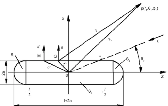
We discern the ideal non-analytical scatterer in the form of the terminal cylinder with the semi-sphres on its ends (see Figure 1).

The pressure p rs

(

1; ;θ ϕ1 1

)

in the scattered wave in the point observation

(

1; ;1 1

)

P r θ ϕ is equally [1] [2] [3] [4] [5]:

(

1; ;1 1

) (

1 4π

)

{

( )

exp

( )

( )(

)

exp

( )

}

d ,

s s s

S

p r θ ϕ =

∫ ∫

_∂p Q ∂n_ ikr r−p Q ∂ ∂n _ ikr r_ S (1)

where Q—the point of the surface of the scatterer.

Then (1) for the Dirichlet condition at the surface is accepting the appearance:

How to cite this paper: Kleshchev, A.A. (2016) Some Methods of Solution of Prob-lems of Sound Diffraction on Bodies of Non- Analytical Form. Open Journal of Acoustics, 6, 45-70.

http://dx.doi.org/10.4236/oja.2016.64005

Received: May 12, 2016 Accepted: December 12, 2016 Published: December 15, 2016

Copyright © 2016 by author and Scientific Research Publishing Inc. This work is licensed under the Creative Commons Attribution International License (CC BY 4.0).

[image:2.595.204.543.65.279.2]

Figure 1. The non-analytical smooth scatterer in the form of the cylinder with the semispheres.

(

1; ;1 1

) (

1 4π

)

{

( )

exp

( )

( )(

)

exp

( )

}

d

D D

s s i

S

p r θ ϕ =

∫ ∫

_∂p Q ∂n_ ikr r+p Q ∂ ∂ n _ ikr r_ S (2)

For the Neimann’s condition:

(

1; ;1 1

)

(

1 4π

)

{

( )

exp

( )

( )(

)

exp

( )

}

d

N N

s i s

S

p r θ ϕ = −

∫ ∫

_∂p Q ∂n_ ikr r+p Q ∂ ∂n _ ikr r_ S(3)

The function Ψ = ∂

(

pΣ ∂n′

)

we are find from the solution of the non-homogeneous Fredholm equation of the second kind [1] [2] [3] [4] [5]:

( ) (

1 2 3; 3; 3

) (

1 4π

)

( )(

)

exp

( )

3 3 d

(

)

exp

( )

3 .

S

r θ ϕ Q n′  ikr′ r′ S n′ i

Ψ −

_{∫ ∫}

Ψ ∂ ∂ _{ } = ∂ ∂ kr (4)

The integral to the left of (4) must understand in the sense of the main meaning. With the help Ψ we are find and the scattered pressure D

s

p in the any point of the medium P r

(

1; ;θ ϕ1 1

)

:

(

1; ;1 1

) (

1 4π

)

( )

exp

( )

d .

D s

S

p r θ ϕ =

∫ ∫

Ψ Q _ ikr r_ S (5)

For the Neimann’s condition, we are bring the function Φ =pΣ—the solution of the

Fredholm equation of the second kind [1] [2] [3] [4] [5]:

( ) (

1 2 3; 3; 3

) (

1 4π

)

( )(

)

exp

( )

3 3 d exp

( )

3 .

S

r θ ϕ Q n′  ikr′ r′ S i

Φ +

_{∫ ∫}

Φ ∂ ∂ _{ } = kr (6)

The scattered pressure in the point P r

(

1; ;θ ϕ1 1

)

we are express through the function Ф:

(

1; ;1 1

)

(

1 4π

)

( )(

)

exp

( )

d .

N s

S

p r θ ϕ = −

∫ ∫

Φ Q ∂ ∂ n _ ikr r_ S (7)

The scattered pressure

(

1; ;1 1

)

D s

The surface S consists of S2 and the surfaces S1 и S3 (see Figure 1).

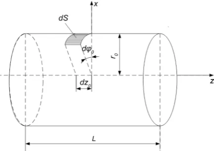
For the calculation of the integrals (2), (3) and (5), (6) on surface S=S1+S2+S3 we are choose the grid of the nodal points [2] [3] [4] [5] (Figure 2, Figure 3).

At Figure 4 is present ps

(

r1,θ ϕ1, 1

)

for the chosen parameters by θ0=90  _(the

curve 1 corresponds to method of the T—matrixes, but the curve 2—to the method of the integral equations).

We are going to spread the method of the integral equations, used in [2] [3] [4] [5]

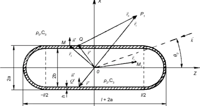
[image:3.595.266.483.278.431.2]

for the ideal non-analytical scatterers, on the elastic shell of the non-analytical form. In the quality of such scatterer, we are going to consider the terminal isotropic elastic cylindrical shell with the semi-spheres on its ends (see Figure 5). The density of the material of the shell is ρ1, the Lame’s coefficients—λ and μ. The shell was filled in the internal liquid medium with the density ρ2 and the sound velocity C3 and it was placed in the external liquid medium with the density ρ0 and the sound velocity C0.

Figure 2. The coordinate system, connected with cylinder.

[image:3.595.295.459.469.687.2]

[image:4.595.281.465.72.307.2]

Figure 4. The modulus of the angular distribution of the scattered pressure.

Figure 5. The elastic shell in the form of the terminal cylinder with the semi-spheres.

At the shell falls the plane harmonic wave with pressure pi under the angle Θ0 and with the wave vector k.

As was shown in [2]-[8], the initial equation is integral equation, having the sense of the generalized Huygen’s principle, for the displacement vector u r

( )

of the elastic shell:

( )

{

( ) (

;

) ( )

ˆ

(

;

)

}

d

( )

, , S

G n S V

′ ′ ′ ′ ′ ′

=

_∫∫

− _ Σ _ ∈

u r t r r r u r r r r r (8)

[image:4.595.203.543.348.529.2]

material; G

(

r r′;

)

is the displacement Green’s tensor; Σ

( )

r r′; is the stress Green’s tensor; if r _{concerns to the point of the surface S, in the left part of the Equation (8)} will stand u r

( )

′ 2.

The second integral equation presents the Kirchhoff integral for the diffracted pres-sure pΣ

( )

P1 in the external medium [2] [9]:

( ) ( )

{

( )(

)

(

)

(

)

2

( )

}

( )

1 1 exp 0 0 exp 0 0 0 d 4π 1 ,

a

a i

S

C P pΣ P = −

∫∫

pΣ Q ∂ ∂n′  ikr r   − ikr r ρ ω un′ S + p P (9)

where pΣ

( )

P1 = p Pi

( )

1 +ps

( )

P1 ; ps

( )

P1 is the scattered pressure in the point P1; C(P1) is the numerical coefficient, equal 2π, if P1∈Sa and 4π, if P1 out Sa; Sa is the

ex-ternal surface of the shell; Q is the point of the exex-ternal surface of the shell.

For the pressure p2

( )

M1 in the internal liquid medium in the point M1 is got the third integral equation:

( ) ( )

{

( )(

)

( )

( )

2

( )

}

1 2 1 2 exp 3 3 exp 3 3 0 d ,

b

b S

C M p M =

∫∫

p Q′ ∂ ∂n′ _ ikr r _{ }− ikr r_ρ ω un′ S (10)

where Q′ is the point of the internal surface of the shell;

( )

1

1

1

4π, if out ;

2π, if ;

b b M S C M M S  =  _∈ 

Sb is the internal surface of the shell.

To the integral Equations (8), (9) and (10) are added the boundary conditions on the external (Sa) and internal (Sb) surfaces of the shell [2] [3] [4] [5] [6].

For choosing boundary conditions we will have the integrals of the two types: the in-tegrals with the isolated special point and the inin-tegrals which are considered of the sense of the principal meaning. The method of the calculation of the second types was described in [2].

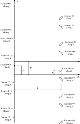
Applying the normal modes and image sources methods for a harmonic signal in the planar waveguide is equivalent [10]. Harmonic signal in the plane waveguide was stu-died previously enough at the great length [2] [11] [12]. At the basis of the imaginary sources and imaginary scatterers method the problem of scattering of the pulse signals on elastic spheroidal bodies is solved, accommodated in the plane waveguide with the ideal boundary conditions. The impulse signals put the energy, therefore they are propagated with the group velocity, which lies in the principles of the imaginary sources and imaginary scatterers method (method of normal waves of the waveguide is not applicable in this case). Temporal and spectral characteristics of the pulse signals reflected and diffracted from the spheroidal shape elastic bodies are obtained for the first time in this paper.

The spectrum S0

(

2πν

)

of the sound pulse of the source with the harmonic filling has the following appearance [13]:

(

)

₍

0

₎

( )

0 _{2 2}

0 0

2π 1 sin π ,

π

n

i

S ν ν nν

ν

ν ν

 

= − _{ }

−   (11)

oscilla-tion periods of the harmonic signal in the pulse; ν —the circular frequency.

The spectrum S0

(

2πν

)

is connected with Ψi

( )

t of the source by the return

Fourier transform:

( ) ( )

1

(

)

(

) (

)

0 0

π Re 2π exp 2π d 2π

i t S ν i ν ν

∞ −

Ψ =

_∫

+ (12)

The spectrum of the scattered (reflected or transmitted) signal Ss

(

2πν

)

is by the product of the spectrum S0

(

2πν

)

at the corresponding meanings of the angular cha-racteristic of the scattering of the spheroidal shell D

(

η ϕ ν, ,

)

(η and ϕ—the angu-lar coordinates of the point of the observation). The spectrum diffracted signal

(

2π

)

SΣ ν depends on S0

(

2πν

)

and Ss

(

2πν

)

.

Similarly to (23) with the use of SS

(

2πν

)

and SΣ

(

2πν

)

images of ΨS

( )

t′ and

( )

t

Σ ′

Ψ —scattered and diffracted pulses respectively [2]

( )

(

)

2π

(

)

0

1

Re 2π e d 2π

π

i t

S t SS

ν

ν ν

∞

+

′

Ψ =

_∫

₍₁₃₎

( )

(

)

2π

(

)

0

1

Re 2π e d 2π

π

i t

t S ν ν ν

∞

+

Σ ′ Σ

Ψ =

_∫

(14)

Considering the elastic shell into the liquid layer with the thickness H and the con-stant sound velocity the boundary conditions will be at follows: at the upper boundary of the waveguide Dirichlet condition is fulfilled, at the lower boundary—Neumann condition [2] [3] (Figure 6).

The scatterer centre is fixed at the distance of z1=0.5⋅H from the bottom and at the horizontal distance R; the point-source Q of the impulse sound signal is placed the depth H−z0=0.5⋅H from the centre (Figure 6).

The scattered field for the non-analytical form elastic shell has been determined ei-ther with the help of the method of the integral equations [2] [3] [14]. As such a scat-terer here the terminal isotropic elastic cylindrical shell with the semi-spheres on its ends (see Figure 5) is going to be considered.

3. Method of Green’S Functions for Ideal Scatterer

We consider non-analytical body, the surface of which does not apply to coordinate symones with divided variables in the scalar Helmholtz equation. We examine this non-analytical scatterer in the form of a finite circular cylinder bounded on the sides of the hemispheres (Figure 1).

[image:7.595.233.512.75.505.2]

Figure 6. The mutual disposition of the impulse point-sources and scatterers in the plane waweg.

( )

1

( )

(

)

( ) ( )

, , d

4π

S

S _S S

p Q

p P p Q G P Q G P Q S

n n

∂

 ∂ 

= _ − _

∂ ∂

 

∫

(15)

where ps(P)—the sound pressure scattered by the body, P—the point of observation, which has a spherical coordinates: r, ,θ ϕ; Q—the point of the surface S; ps(Q)—the sound pressure in the point Q; G(P, Q)—Green’s function of the free space, satisfying the inhomogeneous Helmholtz equation.

In the (15) Green’s function is selected as a potential point source:

(

)

e

,

ikR

G P Q R

= (16)

where k=2π λ—the wave number, λ—the length of a sound wave in the liquid

en-Source 02 (-) (Imag.)

Source 01 (+) (Real) Source 05 (-)

(Imag.)

Source 03 (+) (Imag.)

Source 04 (-) (Imag.) Source 06 (+)

(Imag.)

Source 07 (-) (Imag.)

Source 08 (+) (Imag.) Source 09 (+)

(Imag.)

Scatterer 01 (Real)

Scatterer 03 (Imag.) Scatterer 02

(Imag.) Scatterer 05

(Imag.)

Scatterer 04 (Imag.)

Scatterer 07 (Imag.)

Scatterer 08 (Imag.)

Scatterer 06 (Imag.) Scatterer 09

vironment, R—the distance between the points P and Q.

Using relative arbitrariness of the choice of Green’s function, you can get the Kir-chhoff formula options, consisting of a single member:

( )

1

( )

( )1

₍

₎

, d

4π

S _S S

p P p Q G P Q S

n

∂ =

∂

∫

(17)

( )

1

( )

( )2

₍

₎

, d

4π S

S _S

p Q

p P G P Q S

n

∂ = −

∂

∫

(18)

By using formulas (17), (18) is considerably simplified computational procedure: you want to define only one of the parameters (ps(Q) or dps(Q)/dn) on the surface S. How-ever, in this case, the match of the surface S with a coordinate the surface one of coor-dinate systems in which it is possible separation of variables is necessary. Thus, applica-tion of Green’s funcapplica-tions for analytical surfaces (infinite cylinder and sphere) faces of these surfaces, interconnected is the main feature of this method.

The possibility of such a method and test calculations of the scattered field were con-sidered in [23] [24]. For example, an experiment at the decision of a test problem [23]

for the calculation of the far field of a point source (group of point sources) directly and through (17), (18) has shown that in the considered range of wave sizes of the results obtained by these two methods, good enough coincide. When solving the problem of diffraction to determine the values of ps (Q) and dps(Q)/dn on the surface S you can use the following expression:

1) For the homogeneous Dirichlet conditions (ideally soft body), pressure scattered waves on the surface S have the form:

( )

( )

s i

p Q = −p Q (19)

2) For the homogeneous Neumann conditions (ideally rigid body):

( )

( )

,

i s

p Q p Q

n n

∂ ∂

=

∂ ∂ (20)

where p, (Q)—the sound pressure of the incident wave in point Q. When determining the values pt(Q) you can use the expression for the scalar potential of the plane mo-nochromatic wave single amplitude of the incident on the body from a source located at infinity.

This potential for a perfectly reflective sphere is natural functions in solving the Helmholtz equation in a spherical coordinate system has the following form [6]:

(

) (

₍

)

₎

(

) ( )

0 0

!

( , , ) 2 1 cos cos ;

! n

n m

i n n n

n m

n m

p r i n m P j kr n m

θ ϕ ∞ ε − ϕ θ

= =

−

= +

+

∑ ∑

(21)

(

)

(

)

1 0 ; 2 0 ;

n n n n

ε = = ε = ≠

The expression (21) is simplified when considering the axis-symmetric problem (de-pendence on the coordinate ϕ

( )

(

) (

) ( )

0

, m 2 1 cos ,

i m n

m

p rθ i n P θ j kr

∞ − =

=

∑

+ (22)

plane harmonic waves unit amplitude of the wave vector, k,aimed at the angle θ0 to the z axis of the cylinder, folding natural functions solutions to the Helmholtz equation in a circular cylindrical coordinate system:

(

)

(

)

( )

( )

_{( )}

(

)

( )

₍

₎

1 0 0

0 0 1

0 _{0 0}

sin

, , exp cos 1 cos ,

sin

m m

i m m

m _m

I kr p r z ik z H kr m

H kr

θ

ϕ θ ε ϕ

θ ∞

=

Ω

= − −

Ω

∑

(23)

In the case of the plane problem of the wave vector к perpendicular to the z axis of the cylinder and expression (23) is simplified [6]:

( )

( )

( )

_{( )}

(

)

( )

₍

₎

1 0 0

1

0 _{0 0}

sin

, 1 cos ,

sin

m m

i m m

m _m

I kr p r H kr m

H kr

θ

ϕ ε ϕ

θ ∞

=

Ω

= − −

Ω

∑

(24)

4. Results of Numerical Experiment

For calculation of integral (17) and (18) on the surface S the quadrature formulas is used. A step of integration over the surface S in the axial and circumferential directions

(

dz d0, ϕ θ0,d 0

)

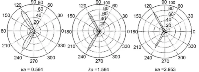
in the system of nodal points must not exceed 0.5λ (Figure 2 and Fig-ure 3).

Using the method of Green’s functions were calculated the equivalent radius Req of

[image:9.595.206.545.396.521.2]

the ideal non-analytical body for several values of wave size ka (where a is the radius of cylinder and hemispheres of the non-analytical scatterer) and different angles of irradi-ation (Figures 7-9).

Figure 7. Angular diagrams Req at the angle of the incident θ0=90

_.

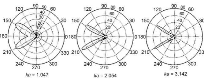
Figure 8. Angular diagrams Req at the angle of the incident θ0=60

[image:9.595.205.549.557.682.2]

[image:10.595.204.538.65.195.2]

Figure 9. Angular diagrams Req at the angle of the incident θ0=30

_.

The analysis of equivalent radiuses Req presented on these pictures, permit to make the following conclusions:

1) The angular position of reflecting and diffraction lobes totally correspond to the physical representations;

2) The angular characteristics Req of submarine non-analytical object are rather simi-lar to the angusimi-lar diagrams of spheroid bodies [2] [25].

At all figures clearly observed diffraction (shadow) petal, and it grows and shrinks with increasing frequency. On Figures 7-9, the mirror petal is shows, which is similar to the shadow petal with increasing frequency, but in contrast, limited asymptotically. You may notice that the angular diagrams of the non-analytical scatterer are very simi-lar to the angusimi-lar characteristics of the scattering elongated spheroids (ideal and elastic) with the ratio of the semi-axes 1:10 [2] [17] [25] [26]. In contrast to works [18], which used a method of integral equations and were calculated for non-analytical body with short cylindrical insert, in this study cylindrical insert was much longer. Values equiva-lent radius at other angles of incidence is given in works [27] [28].

5. Green’s Functions Method for Elastic Scatterers

The solution of the problem of the sound scattering by an elastic shell of the non- analytical form is based an article [29]. The Green’s functions method is approximate because it does not take account the interaction between individual elements forming a compound body of non-analytical form. The interaction between scatterers shaped as spheroids and elliptic cylinders in [2] and this interaction was negligibly small. In addi-tion, the sound scattering characteristics calculated for bodies with mixed boundary conditions by the Green’s function method namely the Sommerfeld method (the me-thod of un-determined coefficients [2] [25]), and the agreement between the results was fairly good.

As non-analytical bodies considered two structures:

1) A finite-length circular cylindrical elastic shell limited an the ends by the two halves of a prolate spheroidal shell (Figure 10);

[image:11.595.232.519.68.189.2]

Figure 10. The cylindrical shell with the semi-spheroidal shells.

In article, [29] gave a decision acoustic scattering problems to the constituent parts of no analytical bodies. For cylinder and spheroidal shells are used Debye and Debye-type potentials. In [29] the angular scattering characteristics of such com-pound bodies with different wave sizes are calculated.

We consider a compound elastic shell formed by a finite cylindrical shell whose ends are closed by two hemi spherical shells of the same diameter (Figure 5). To apply the Green’s function method, it is necessary to take the solution to the axi-symmetric problem of plane wave diffraction by an elastic spherical shell in terms of dynamic elas-ticity theory [30] and transform this solution to the three-dimensional version. The re-sulting solution little differs from that obtained above for the three-dimensional prob-lem of diffraction by a spheroidal elastic shell [2] [25] [26] [31].

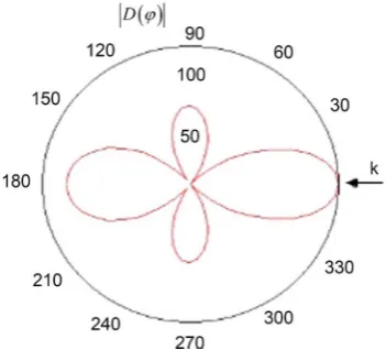
Figure 11 and Figure 12 show the absolute values of the angular characteristics

( )

D ϕ (in the XOY plane, θ0 =90

_{) for non-analytical elastic scatterer in the form of}

a cylindrical shell connected with to spherical shells (Figure 3) the following parame-ters: ka = 0.523 (Figure 11) and ka = 0.941 (Figure 12).

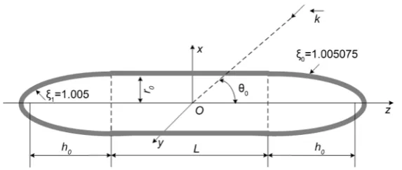
The method of Green’s functions in combination with analytical methods can be used for the solution of tasks of diffraction of plane sound wave on elastic isotropic scatter of non-analytical form, that consists of circular cylindrical shell of terminated length L and radius r0, bounded at the butts by the halves of elongated spheroidal shell

[28] (Figure 10).

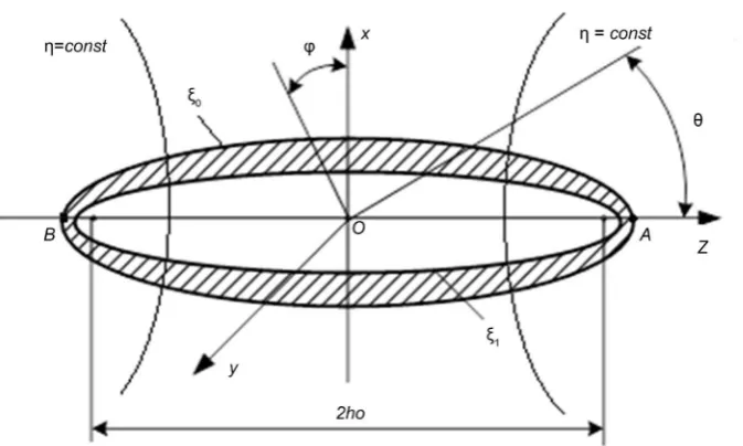
The internal surface of the spheroidal shell is given by coordinate ξ =1 1.005 (with the proportion of the axes of the inner spheroid 10:1 and inter-focal distance 2h0), and external-by coordinate ξ =0 1.005075.

The shell material is isotropic, with the density ρ1, coefficients of Lame λ1 and µ1, module of Jung E, inside is the gas with density ρ2, coefficient of volumetric compres-sion K2 and sound rate с2.

The scatterer is placed in ideal compressed liquid with density ρ0 and coefficient of volumetric compression K0. The potential of sound wave is submitted to scalar equa-tion of Helmholtz.

[image:12.595.282.462.76.242.2]

Figure 11. The modulus of an angular characteristic.

Figure 12. The modulus of an angular characteristic.

elastic cylindrical surface and elastic spheroidal surfaces, respectively.

The schemes of solution of axially symmetric tasks of diffraction on elastic cylinder and spheroid are rather similar: in both cases the vector potential Ψ has the single nonzero component Ψ = Ψϕ. The unknown coefficients of potentials’ expansion of

falling and dispersed waves, of scalar potential of the surface, of potentials of Debye U and V, as well as of potential of gas, filling the surface, are found from the physical boundary conditions on the external and internal surfaces of the shell [32].

Although on the spheroid these coefficients are found not in the enclosed form, but using the method of truncation from the infinite system of equations.

What is more, while finding the solution of tridimensional task of diffraction on elas-tic speroidal scatterer the vector potential Ψ is presented by the potential of Debye U and V [2] [19] [32]:

(

)

2

(

)

,

rot rot U ik rot V

= R + R

Ψ ₍₂₅₎

[image:12.595.285.461.277.436.2]

The sound pressure in the far-field can be found by one of the numerical methods, among those is the comfortable method based on the usage of mathematical formula of Helmholtz-Huygens ‘Principle (integral of Kirchhoff) [25]:

(

1 1 1

) (

)

( )

( )

( )

( )

exp exp

; ; 1 4π d

s s s

S

ikr ikr

p r p Q n p Q s

r r r

θ ϕ = _∂ ∂  − __∂∂ _ _

 

 

∫∫

(26)

where r—is the distance between the point Q on the surface of the shell and the point P with coordinates r1, θ1, φ1 in the far-field.

The Green’s functions in (26) are taken in the form of potential of the point-source. The quadrature formulas are used for finding of this integral, and here the integration step (sampling) of the surface of the scatterer should not exceed 0.5λ0, where λ0—is the length of the plane monochromatic wave, falling from the liquid onto the surface of the scatterer.

The Green’s functions in (26) are taken in the form of potential of the point-source. The quadrature formulas are used for finding of this integral, and here the integration step (sampling) of the surface of the scatterer should not exceed 0.5λ_{0, where} λ_{0—is the} length of the plane monochromatic wave, falling from the liquid onto the surface of the scatterer.

6. Methods of Kupradze, T-Matrix and Geometrical

Theorie of Diffraction

The other way of solving the task of sound diffraction on elastic isotropic body with non-analytical surface is based on the method of Kupradze [16]. According to this me-thod the scattered pressure p rs

( )

and the vector of displacement of elastic body

( )

u r can be presented in the form of potentials, focused on the surface of the elastic body S:

( )

0

(

) ( )

d ;

s s

S

p r =

∫∫

G r−r′ p r′ S (27)

( )

(

) ( )

d ,

S

G ′ ′ S

=

_∫∫

−

u r r r u r (28)

where r′—is the radius-vector of the surface point S; ps

( )

r′ and u r

( )

′ —are the

unknown scalar and vector densities, the function G0 and matrix G differ from the Grin function of Helmholtz’ operator and from the tensor of displacements of Grin by the constant multipliers:

( )

( )

(

) ( )

(

)

{

( )

( )

( )

}

( ) ( )

(

)

( ) ( )

( )

1

1 _{2 2}

0 1 2

1 1

2 1

exp ; 1 ;

exp ; exp .

T T L

T L

G ik G k A A A

A ik A ik

ρ ω −

−

− −

= = + ∇∇_ _−

= =

r r r r r r r

r r r r r r

(29)

From the common characteristics of wave and elastic potentials we find that ps

( )

r′

and u r

( )

′ satisfy the system of the four integral equations on the surface S:

(

) (

) (

)

(

)

_{1 2}

2

1 ps n pi n 2π ;ps n ps pi 2π ;un τ 0; τ 0,

ρ ω u n⋅ = ∂ ∂ + ∂ ∂ − σ = − + − σ = σ = (30)

the dash means that the called direct values of these parameters. The numerical so-lution of the system (16) on computers for elongated elastic bodies is marked by consi-derable processing difficulties. The asymptotic methods, permitting to get the approx-imate solutions of the system (14) are used in (16); these methods are based on asymp-totic formulas for integrals, received in [17].

The usage of method of T-matrix in the task of sound diffraction on elastic bodies of non-analytical form is examined in [11]. The source system of integral solutions for the displacement vector u r

( )

of elastic finite cylinder with spherical shell plates (Figure

1) is got with the help of [19], and the integral equation for uΣ

( )

x substitutes the

integral of Kirchhoff:

(

1; ;1 1

) (

1 4π

)

( )

exp

( )

exp d .

s

s s

s

p Q ikr ikr

p r p Q S

n r n r

θ ϕ = _∂ − ∂ _ __

∂ ∂  

 

∫∫

(31)

The equation for uΣ

( )

x is received from (1) with addition of vector of

displace-ment u xi

( )

in the falling wave, and with conversion of module of displacement in the

expressions for tensor of stress of Cauchy T x

( )

and tensor of stress of Grin Σ

(

x x′;

)

in nil. As the result, the second integral equation gets the form of [17]:

( )

( )

(

;

)

( ) (

;

)

d

( )

( )

,

i S

G S

Σ Σ

 ′ ′ ′ ′ ′  ′

−

_∫∫

_ ⋅_ ⋅Σ _− ⋅ _ =

u x u x n x x t x x x x u x (32)

where the vector x refers to the point of fluid medium, outside the surface S. The solution of the received system of the two integral equations is found by the me-thod of T-matrix with the use of boundary conditions.

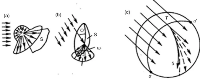
The particular place in the tasks of diffraction on the bodies with non-analytical sur-face in the sphere of high frequencies is occupied by the geometrical theory of diffrac-tion (GTD), based on the asymptotic methods [2] [33].

In comparison to ray acoustics (RA), the GTD regards the process of formation of diffraction rays along with reflection and refraction. When the wave falls onto the body or its edge, the boundary shade-light appears for geometrical rays, i.e. the geometro- acoustic solution faces the break that states the formation of additional diffraction fields, compensation this break.

The four main additional laws are considered in GTD, in comparison to RA: two of them determine the direction of diffraction rays, two others—their amplitudes:

1) The range of diffraction rays is produced not by all of the falling rays, but:

а) by the rays falling onto the non-homogeneous parts of the body S—edges, ridges, lines of discontinuity in the curvature (Figure 13(a) and Figure 13(b)); b) by the rays contacting the body (Figure 13(c)).

2) When the ray of the primary field falls onto the edge of the body (Figure 13(a)), the diffraction rays radiate from it in all the directions, forming the spherical wave. If the ray contacts the ridge (Figure 13(b)), the diffraction rays form the cone in its each point. The angle ω of cone opening is equal to the angle Ω _{between the tangent to}

the ridge and the falling ray, what means,

[image:15.595.202.541.76.210.2]

Figure 13. The varieties of diffraction fields in the terms of geometrical theory of diffraction.

The law of formation of diffraction rays in the sphere of shade of plain convex body differs from the law of rays’ formation at edges and ribs. In this case, the diffraction rays get away from the surface of the shade part of the body and form the slippage waves.

Each ray of the falling wave which contacts the body, from the “surface ray” T−b (Figure 13(c)) on the surface of the body, that is the geodesic (shortest) line on the surface of the body. The direction of the ray in point T of the horizon aa′, i.e. at the point of formation, coincides with the direction of the falling ray. The number of the rays of slippage wave gets tangentially off the range of surface rays.

3) The amplitude of diffraction ray is proportionate to the amplitude of the format-ting primary ray in the impact point. The diffraction fields can be presented in the formula:

(

_i

)

(

_i,

)

exp

( )

,

u_Σ = u J D t t_Σ ikS (34)

where S—is the eikonal (function, determing the phase structure of the field—the sys-tem of the wave front); J—is the Jacobian of transition to the ray coordinates—the pa-rameter, proportionate to the area of cross-section of rays of the tube; t ti, Σ—the gra-dients of the falling and diffraction rays;

u

i—the amplitude of the falling wave: in the

point of the edge or the rib, where the concerned ray originates, or on the point of the horizon, where the surface ray producing the concerned diffraction ray, appears.

The parameter D

(

t ti, Σ

)

is named the coefficient of diffraction. It is received re-garding the fourth law of GTD.

4) The coefficient (matrix) of diffraction D is determined by local features of body’s geometry in the area of the falling ray (in the case of edges and ribs) or in the area of the surface ray between the falling point and take-off point of diffraction ray (in the plain body).

In terms of physics D

(

t t_i, _Σ

)

—is the amplitude of the source, corresponding to the ray that gets off on the direction tΣ in the case of the falling of the plain wave with

singular amplitude in the direction ti.

produc-es diffraction rays, then the amplitude of diffraction field will not be equal to zero, i.e. the formula (18) cannot be used. In this case the diffraction field will be proportionate to the value of the first derivative of the amplitude of the primary field along the front.

The algorithm of solution of the task of diffraction consisting of 3 rules is based on the laws of GTD:

1) The solution is found as the result of number of the fields of ray type:

(

)

exp .

n n n

n n

u=

∑

u =

∑

A ikS (35)

One of the components is the primary field. Each of the fields differs from zero in the area with the boundary of the body surface and the shade-light boundary of the field. 2) All the sum (33) components, except the primary field (it is considered to be

de-fined) are determined from the primary field according to the laws of RA and of GTD.

It should be kept in mind that the reflected, refracted and diffraction fields can be formed from the primary field not only directly but also as the result of the complex sequence of reflections, refractions and diffractions.

1) The question of the choice of the coefficients of diffraction is important in the process of calculations of diffraction fields. According to the fourth law of GTD, the coefficients of diffraction are equal to all bodies that possess equal local geometrical features and the features of geometry of the falling wave. Here logically appears the third rule of algorithm of diffraction task.

2) The coefficient of diffraction in the present task is found from the analysis of the precise solution of the simple (model) task, close in geometry. For example, in the case of diffraction of the field Φ =Aexp

( )

ikS on the curved opening in non- plane screen the model task is the task of diffraction of the plane wave on semi- surface, touching the surface of the screen and the edge of the tip in the examined point.

The usage of GTD is limited in the present number of solutions because the coeffi-cients of diffraction D are determined in the model tasks. In the present the model tasks for numerous two-dimensional cases-fir diffraction on the wedge, plain cylinder, etc.— are solved. In the model three-dimensional tasks, we frequently have to use the ap-proximate results.

7. Method of Finite Elements

The method of the finite elements (MFE) and its variations allow getting the solutions of tasks of sound radiation of elastic bodies of nearly all forms. Here we consider, for example, the possibility of common use of MFE with the method of Grin functions for numerical solution of task of the distant field of sound radiation by extended spheroid shell, under the influence of the point sources on its surface (Figure 14):

[image:17.595.207.544.66.268.2]

Figure 14. Extended spheroid shell, under the influence of the point sources on its surface.

diffraction of plane monochromatic wave on this shell; the solution is presented in [18] [34]. This task can be interpreted as the task of sound radiation of elastic body under the influence of turbulent pulsations of liquid flow, and the calculation based on the focused force that is stipulated by this pulsation, presents certain interest. In this case, it is useful to compare the results of the numerical solution with analytical solution re-sults for valuation of its accuracy.

The geometrical and physical parameters of the shell are similar to those presented on Figure 14. The point sources of harmonic signal are situated at the ends of the shell at the points A and B; these sources imitate the turbulent pulsation and produce some amplitude-phase distribution (AFD) of the sound wave potential on the external sur-face ξ0 and in the liquid surrounding the shell.

The numerical solution of the task is made in two stages [18]:

1) The calculation of the values of sound wave potential and its gradient on the closed test area in the nearest field (of the Fresnel zone), that are created by the point sources;

2) Re-calculation of received results in the distant field (in the Frauenhofer zone). On the first stage it is necessary to conjugate the solutions of FEM on the surface of area S in the sphere V1, adjoining the shell, with the point analytical solution of equa-tion of Helmholtz in the external endless sphere V2 (Figure 15).

The functional of the full energy if the system “shell-fluid” will have the form:

(

)

0

(

)

1 2 0 1 1 0 1 2

, , d d d ,

2

s s s

E w P T i w S S S

v v

ρ

ωρ ∂Φ∑ ρ ∂ΦΣ

Φ Φ = + − Φ + Φ + Φ − Φ

∂ ∂

∫∫

∫∫

∫∫

(36)

[image:18.595.197.550.75.238.2]

Figure 15. The conjugation of FEM with the point analytical solution.

The condition of stationary state of E functional leads to fulfillment of equation of the shell movement and of equation of Helmholtz in the sphere V1, as well to equality of the normal speeds 1

v

∂Φ ∂ and

2 v

∂Φ

∂ and potentials Φ1 and Φ2 on the surface S. The axial symmetry of the shell and sources of radiation leads to the fact that the dis-placements of the shell and potentials of liquid speed will not be subject to the sur-rounding coordinate φ.

The substitution of the forms that approximate the shell displacements and poten-tials Φ1 and Φ2 in conditions of stationary state of E functional leads to the lineal alge-braic system of the solving equations.

For the solving of this task is necessary to use the circular finite elements for: the shell, liquid and filling gas, for conjugation of these elements between one another, as well as the finite elements for modeling of the sphere V2. Using these elements is possi-ble to calculate the nearest field for the arbitrary sources in the form of the shells if spinning. In this case, the numerical calculations are made for the finite-elementary net that consists of 131 elements and 410 focal points (Figure 16).

The AFD of the sound pressure and normal component of vibration speed in the focal points of control surface in the nearest field is initial for the second stage of the task solution.

The sound pressure in the distant field is found with Kirchhoff’s integral, as well as in (26).

The two variants of the forms of control surface were used in the calculations: Non-analytical in the form of cylinder with hemispheres on the edges (as the most useful from the measuring process organization point of view, Figure 17(a)) and ana-lytical (sphere) (Figure 17(b)).

[image:19.595.254.491.70.271.2]

Figure 16. The finite-elementary net in the nearest field of the shell.

(a) (b)

Figure 17. The control surface in the form of: cylinder with hemispheres at the edges (a) and sphere (b).

8. Boundary Elements Method

For the solving of tasks of radiation and diffraction for the bodies of non-analytical surface the boundary element method (BEM) is successfully used during the last years; the numerous scientific works are published on this research area, where the theoretical basis of the method as well as the different aspects of the application are stated [7] [15] [34].

The bibliography analysis shows that BEM is one of the most relevant and widely used among the other numerical methods of solving the boundary tasks.

The following advantages of BEM (in comparison with FEM, for instance) can be considered when solving the tasks:

1) The sampling of the boundary of the sphere with scatterer, not of the whole sphere, when as the result the additional measures for realization of condition of radia-tion at infinity are not demanded;

ξ0

[image:19.595.195.550.301.460.2]

2) The reduction of initial differential equation to the boundary integral equation that presents the exact formulation of the stated task. Here the accumulation of error comes in the process of numerical solution of integral equations in the result of sam-pling, approximation and calculation;

3) The use of analytical method, true for the whole sphere, provides the potentially higher accuracy than FEM does, where the approximation is committed in every area. In the common case for scatterers of general geometric form the boundary surface is presented in the form of collection of elementary areas [2] [18] [34].

The conception of formation of isoparameter elements allows converting the key coordinates of every point of initial elements xiα to the corresponding curvilinear coordinates x ii

(

=1, 2, 3

)

. Here, the element’s geometry (global coordinates) and the main variables (of displacement) are stated using the similar interpolating relations (functions of the form) [18] [34] (Figure 18).

The curvilinear coordinates of every point of the element x i_i

(

=1, 2, 3

)

will be con-nected by the key coordinates xiα in the expressions [2] [18] [34]:

( )

( )

, 1, 2, , 6 or 8

i i

x N_α x_α

α

ξ =

∑

ξ α=  (37)

where N_α

( )

ξ —the functions of local coordinates

( ) (

ξ = ξ ξ₁; ₂

)

—are described shortly:

а) For quadrangular elements:

( ) ( )(

)(

)(

)

( ) ( )(

)(

)(

)

1 1 4 1 1 2 1 1 2 1 ; 2 1 4 1 1 2 1 1 2 1 ; N ξ = ξ + ξ + ξ ξ+ − N ξ = ξ − ξ + ξ ξ− +

( ) ( )(

)(

)(

)

( ) ( )(

)(

)(

)

3 1 4 1 1 2 1 1 2 1 ; 4 1 4 1 1 2 1 2 1 1 ;

N ξ = −ξ ξ − ξ ξ+ + N ξ = ξ + ξ − ξ − +ξ

( ) ( )(

)

(

2

)

( ) ( )(

)

(

2

)

5 1 2 1 1 1 2 ; 6 1 2 2 1 1 1 ;

N ξ = ξ + −ξ N ξ = ξ + −ξ

( ) ( )(

)

(

2

)

( ) ( )(

)

(

2

)

7 1 2 1 1 2 1 ; 8 1 2 1 2 1 1 ;

N ξ = ξ − ξ − N ξ = −ξ −ξ

b) For triangular elements 

( ) (

ξ = ξ ξ ξ1; 2; 3

)

:

( )

(

)

( )

(

)

( )

(

)

1 1 2 1 1 ; 2 2 2 2 1 ; 3 3 2 3 1 ; N ξ =ξ ξ − N ξ =ξ ξ − N ξ =ξ ξ −

( )

( )

( )

4 41 3; 5 41 2; 6 4 2 3. N ξ = ξ ξ N ξ = ξ ξ N ξ = ξ ξ

These correlations present the implicit conversion of surface element to the plane square or the plane equilateral triangle (Figure 18).

The correlations for interpolation of displacements and stress are expressed similarly

[image:20.595.214.535.585.689.2]

(a) (b)

Figure 18. The initial (a) and the corresponding curvilinear isoparameter (b) boundary elements.

ξ1

ξ1

ξ1

ξ1

ξ2 ξ2 ξ2 ξ2

on each element [24]:

( )

( )

;

i i

u Nα uα

α

ξ =

∑

ξ (38)

( )

( )

,

i i

t Nα tα

α

ξ =

∑

ξ (39)

where uiα and tiα—are the parameters of components of vector of displacement or

vector of stress at the nodes.

While submitting (38), (39) in the equation and using the rule of numerical integra-tion, we get

[ ]{ }

H u =   G

{ }

t , (40) where H and G—are the matrix of coefficients used in the result of numerical integra-tion.

Here, we form the integral equation for diffracted pressure basing on (1.15) pΣ at

the view point P1 [2] [17]:

( ) ( )

{

( )(

)

( )

( )

2

(

)

}

( )

1 1 exp exp d 4π i 1 ,

S

C P p_Σ P = −

∫∫

p_Σ Q ∂ ∂n′ _ ikr r_{ } − ikr r_ρω u n⋅ ′ S+ p P (41)

where C P

( )

1 —is the numerical coefficient, equal to 2π, if P1∈S, and 4π, if P1∉S. Now we interpolate the components of the vector u on each boundary element in correspondence with (38); the sound pressure on each element is presented, similarly to (38) and (39), in the form of:

( )

( )

.

p N_α p_α

α

ξ ξ

Σ =

∑

Σ (42)

While submitting (38), (39) and (40) in (41) and completing the numerical integra-tion, we receive

[ ]

T

{ }

u =

[ ]

D

{ }

pΣ +4π

{ }

pi , (43) where T and D—are matrix of coefficients.

On the next stage we solve the system of Equations (40) and (43) using the boundary conditions.

According to the boundary condition the number of indeterminate stress in Equa-tion (40) can be expressed through pressure:

[ ]

H

{ }

u =

[ ]

G t

{ }

+

[ ]

F

{ }

pΣ , (44) where G and F—are matrix of coefficients, received from matrix G in Equation (40).

The distributions pΣ

( )

Q and

(

u n⋅ 1

)

on the surface S are found from Equations (43) and (44), and then the diffracted sound pressure pΣ

( )

P1 in fluid sphere is calcu-lated using (41).

frag-ments of cylinders and spheres (hemispheres).

In the process of numerical integration the element of the surface of cylinder with radius r0 will be equal to S=r0dϕ0dz0; for hemisphere the element of the surface in the spherical coordinates is equal to 2

0 0 0 0

dS=r sinθ θ ϕd d (Figure 2 and Figure 3). In the process of formation of the net of boundary elements for this task, the discre-tization step of the boundary surface in the direction of every coordinate should not al-so exceed 0.5λ0.

According to the theorem of Helmholtz, the displacement vector u can be pre-sented in the form of:

,

grad rot

= − Φ +

u Ψ (45)

where Φ_{—is the scalar,} Ψ_{—is the vector potentials that obey to the scalar and the}

vector equation of Helmholtz, respectively: 2 1 0; k

∆Φ + Φ = (46)

2 2 0, k

∆ +Ψ Ψ= (47)

where k1=ω c1; k2=ω c2 ; c1 and c2—are velocities of linear and transverse waves respectively in the material of the scatterer.

For cylinder surface the vector Ψ _{is parallel to axis of cylinder, i.e. т.е.}

, 0.

z ϕ r

Ψ = Ψ Ψ = Ψ =

Due to the axis symmetry of the task for spherical surfaces the vector potential Ψ

will also have the only one component Ψϕ, different from zero: Ψ = Ψϕ, in the

spherical coordinate system. Thus, the vector equation of Helmholtz (47) transfers into scalar equation for the only component of vector potential, different from zero:

2 2 0. k

∆Ψ + Ψ = (48)

The potential of diffused wave, as well as the potentials Φ и Ψ are taken in the forms, corresponding to the plane wave and containing the voluntary constants that are determined from the boundary conditions.

While all the main physical variables are functions of only two coordinates, the dis-placement vector would also possess two components.

Using the correlations of the generalized law of Hooke for isotropic sphere, not de-pending of the choice of coordinate systems, it is possible to present the elastic stress on the finite surface through the deformation components, and then through potentials

Φ _and Ψ _{[2] [25]:}

а) For cylindrical surface:

2 2

2 2 1

1 1 2 2 ;

r k r r

r r

σ λ µ

ϕ ϕ

− −

 ∂ Φ ∂Φ ∂ Φ 

= Φ + _− − _

∂ ∂ ∂

∂

  (49)

2 2

1 2 2

2 2

2 2 2 ,

r r r k

r r

ϕ

τ µ

ϕ ϕ

− −

 ∂ Φ ∂Φ ∂ Ψ

= _− + − Ψ − _

∂ ∂ ∂ ∂

  (50)

where ϑ ε= r+εϕ =divu;

1 1

ctg ;

r

u r r

r θ θ

− −

∂Φ ∂Ψ

= − + Ψ +

∂ ∂ (51)

2 2

2 1 2 1 2

1 2 2 ctg ctg ;

r k r r r r

r r r

r

σ λ µ θ θ

θ

− − − −

 ∂ Φ ∂Ψ ∂ Ψ ∂Ψ

= Φ + _− + − Ψ + − _

∂ ∂ ∂ ∂

∂

  (52)

2 2

2 2 2 2 2

2 2

ctg 2 sin ,

r r r r r

r

θ

τ µ θ θ

θ θ θ

− − − − −

 ∂Ψ ∂ Ψ ∂ Ψ ∂Φ 

= _ + − − − Ψ _

∂ ∂ ∂ ∂

  (53)

where ϑ ε= r+εϕ =divu.

The following boundary conditions are to be executed at the points of the boundary surface:

a) The normal (radial) component of the displacement vector ur is continuous and

connected with normal derivate of diffracted pressure pΣ = pi+ ps:

1 2 0 r p u n ρ ω− − ∂ Σ

=

∂ by r=a, (54) where p pi, s—are the sound pressures of the falling and dispersed waves respectively;

the normal stress σr is equal to acoustic pressure in liquid:

r p

σ = Σ by r=a; (55)

b) The pressure tangents are missing:

0 rϕ rθ

τ =τ = by r=a. (56)

While submitting the component of the displacement vector and elastic stress to the boundary conditions (54)-(56) we receive the algebraic systems of equations for every point on the surface for finding out the indeterminate coefficients in equations of po-tentials Φ and Ψ.

The indeterminate coefficients are received using the ratio of determinants by the rule of Cramer, that allows to receive subsequently the distributions pΣ

( )

Q and ur

at the nodes of the boundary elements.

The calculation of the diffracted sound pressure ps

( )

P in liquid sphere is

processed basing on (26) by numerical integration of quadrature formulas.

The task solution of diffraction for the elastic isotropic surface does not differ in principle from the examined solution for constant elastic body: the internal boundary (with filler or vacuum inside the shell) is added, and thus the number of indeterminate coefficients and the number of boundary conditions in (49)-(56) increase.

The additional boundary conditions are formed the following way:

4) The normal stress on internal surface of the shell is either missing (the hollow shell) or is equal to the sound gas pressure (gas filled shell);

5) The absence of the tangent stress on internal surface of the shell.

[image:24.595.204.546.70.253.2]

(a) (b)

Figure 19. Modules angular characteristics of spherical scatterers (BEM) when ka = 1, Req:(a) solid sphere: 1—tight; 2—steel; 3—aluminum; 4—rubber; (b) spherical shell of thickness h: 1 − kh = 0.01; 2 − kh = 0.03; 3 − kh = 0.05; 4 − kh = 0.1.

(a) (b) (c)

Figure 20. Modules angular characteristics of spheroids, Req: 1—steel (exact solution); 2—steel (BEM); 3—rubber (BEM); (a) for C = 3; (b) for C = 5; (c) for C = 10; (where C=kh0).

Also the results of calculations of scattered characteristics for elastic scatterer with non- analytical surface form (cylinder with hemispheres at the edges), by FEM, are presented there; the results were approximate to the corresponding results of the precise solution for spheroids, received in [2] [25].

9. Conclusions

The article analyzes seven methods of the solution of the problem of the sound scatter-ing on ideal and elastic bodies of the non-analytical forms: method of integral equa-tions, method of Green’s funcequa-tions, the method of Kupradze, T-matrix method, the method of the geometrical theory diffraction, the method of finite elements and the boundary elements method. This analysis is supplemented with calculations of charac-teristics of the sound scattering by ideal and elastic scatterers of non-analytical forms.

[image:24.595.198.552.316.459.2]

the help with calculations.

Acknowledgements

The work was supported as a part of research under State Contract No. P242 of April 21, 2010, within the Federal Target Program “Scientific and Scientific-Pedagogical Per-sonnel of Innovative Russia for the Years 2009-2013”.

References

[1] Honl, H., Maue, A. and Westpfahl, K. (1961) Theorie der Beugung. Springer, Berlin. [2] Kleshchev, A.A. (2012) Hydroacoustic Scatterers. Prima, St. Petersburg.

[3] Kleshchev, A.A. (2012) Method of Integral Equations in Problem of Sound Diffraction on Bodies of Non-Analytical Form. International Journal of Mechanics and Applications, 2, 124-128. https://doi.org/10.5923/j.mechanics.20120206.04

[4] Kleshchev, A.A. (2013) Method of Integral Equations in Problem of Sound Diffraction on Bodies of Non-Analytical Form. Journal Marine Gazette, 2, 94-98.

[5] Kleshchev, A.A. (1995) Method of Integral Equations in Problem of Sound Diffraction on Elastic Shell of Non-Analytical Form. Journal of Technical Acoustics, 2, 29-30.

[6] Kleshchev, A.A. (1989) Sound Scattering by Ideal Bodies of Non-Analytical Form.

Pro-ceedings of LKI “The Сommon Ship’s Systems”, 95-99.

[7] Seybert, A.F., Wu, T.W. and Wu, X.F. (1988) Radiation and Scattering of Acoustic Waves from Elastic Solids and Shells Using the Boundary Element Method. Journalof Acoustical

Society of America, 84, 1906-1912. https://doi.org/10.1121/1.397156

[8] Podstrigach, J.S. and Poddubniak, A.P. (1986) Scattering of Sound Beams at Bodies of Spherical and Cylindrical Form. Naukova Dumka, Kiev.

[9] Varadan, V.V., Varadan, V.K. and Dragonette, I.R. (1982) Computation of a Rigid Body Scattering by Prolate Spheroids Using the T-Matrix Approach. Journal ofAcoustical

Socie-ty of America, 84, 22-25. https://doi.org/10.1121/1.387311

[10] Grinblat, G.A., Kleshchev, A.A. and Smirnov, K.V. (1993) Sound Fields of Spheroidal Scat-terers and Radiators in Plane Waveguide. Acoustical Journal, 39, 72-76.

[11] Bostrom, A., Varadan, V.K. and Varadan, V.V. (1980) Acoustic, Electromagnetic and Elas-tic Wave Scattering—Focus on the Matrix Approach. Pergamon Press, New York.

[12] Grinblat, G.A. and Kleshchev, A.A. (1994) The Scattering and the Emission of the Bodies Placed in the Plane Waveguide. Journal of Technical Acoustics, 1, 3-6.

[13] Kharkevich, A.A. (1995) Spektrum and Analysis. Springer-Verlag, Berlin.

[14] Kleshchev, A.A. (2015) Diffraction of Pulsed Sound Signals by Elastic Bodies of Analytical and Non-Analytical Forms, Put in Plane Waveguide. Zeitschrift fur Naturforschung A, 6, 419-427. https://doi.org/10.1515/zna-2015-0062

[15] Brebbia, K. and Walker, C. (1982) Application of the Boundary Element Method in Engi-neering. MIR, Moscow. https://doi.org/10.1007/978-3-662-11273-1

[16] Kupradzc, V.D. (1963) Methods of Potentials in the Theory of Elasticity. Fizmatgiz, Mos-cow.

[18] Dushin, A., Il’mcnkov, S.L., Kleshchev, A.A. and Postnov, V.A. (1989) Use of Finite Ele-ment Method to Solution of Problems of Sound Radiating Elastic Shells. Proceedings

Sym-posium “Interaction of Acoustic Waves with Elastic Bodies”, Tallinn, 26-27 October 1989,

89-91.

[19] Peterson, B. and Strom, S. (1975) Matrix Formulation of Acoustic Scattering from Multi-layered Scatterers. Journal of Acoustical Society of America, 57, 2-13.

https://doi.org/10.1121/1.380397

[20] Numrich, S.K., Varadan, V.V. and Varadan, V.K. (1981) Scattering of Acoustic Waves by a Finite Cylinder Immersed in Water. Journal of Acoustical Society of America, 70, 1407- 1411. https://doi.org/10.1121/1.387131

[21] Kleshchev, A.A. (1974) Sound Diffraction on Bodies with Mixed Boundary Conditions.

Acoustical Journal, 20, 632-634.

[22] Kleshchev, A.A. (1984) Accuracy of Green’s Functions Method. Proceedings of LKI

“Acoustics of Ships and Oceans”, 19-24.

[23] Kleshchev, A.A. (1993) Method of Integral Equations for Solution of Problem of Sound Diffraction on Elastic Shell of Non-Analytical Form. Journal of Technical Acoustics, 2, 66- 67.

[24] Il’menkov, S.L. (2014) Green’s Functions Method in Problem of Sound Diffraction on Bo-dies of Non-Analytical Form. Journal Marine Intellectual Technologies, 2, 32-36.

[25] Kleshchev, A.A. and Klukin, I.I. (1987) Principles of Hydroacoustis. Shipbuiilding, Lenin-grad.

[26] Kleshchev, A.A. (2002) Diffraction and Propagation of Waves in Elastic Mediumsand Bo-dies. Vlas, St Petersburg.

[27] Il’menkov, S.L. and Kleshchev, A.A. (2014) Solution of Problems of Sound Scattering on Bodies of Non-Analytical form with Help of Method of Green’s Unctions. Journal

Ad-vances in Signal Processing, 2, 50-54.

[28] Il’menkov, S.L., Kleshchev, A.A. and Klimenkov, S.L. (2016) Green’s Functions Method in Problem of Sound Diffraction on Elastic Shell of Non-Analytical Form. Proceedings of the

15th L. M. Brekhovskikh’s Conference, Moscow, 123-126.

[29] Il’menkov, S.L. Kleshchev, A.A. and Klimenkov, A.S. (2014) The Green’s Function Method in the Problem of Sound Diffraction by an Elastic Shell of Noncanonical Shape. Journal

Acoustical Physics, 60, 617-623. https://doi.org/10.1134/S1063771014060062

[30] Kleshchev, A.A. and Klimenkov, A.S. (2013) Diffraction of Sound Impulses on Isotropic Bodies of Spherical Form (Strict Solution). Journal Advances in Signal Processing, 1, 68-77. [31] Kleshchev, A.A. (2006) Diffraction, Radiation and Propagation of Elastic Waves. Profprint,

St Petersburg.

[32] Kleshchev, A.A. (2012) Debye and Debye-Type Potentials in Diffraction, Radiation and Elastic Waves Propagation Problems. Journal Physical Acoustics, 58, 308-311.

https://doi.org/10.1134/S106377101202008X

[33] Kaminetzky, L. and Keller, J.B. (1972) Diffraction Coefficients for Higher Order Edges and Vertices. Journal Applied Mathematics, 22, 109-134. https://doi.org/10.1137/0122013 [34] Il’menkov, S.L. (2015) Calculation of Sound Scattering Characteristics of Elastic Body of

Non-Analytical Form Using Boundary Element Method. Journal Marine Intellectual

Submit or recommend next manuscript to SCIRP and we will provide best service for you:

Accepting pre-submission inquiries through Email, Facebook, LinkedIn, Twitter, etc. A wide selection of journals (inclusive of 9 subjects, more than 200 journals)

Providing 24-hour high-quality service User-friendly online submission system Fair and swift peer-review system

Efficient typesetting and proofreading procedure

Display of the result of downloads and visits, as well as the number of cited articles Maximum dissemination of your research work