Munich Personal RePEc Archive
Wealth effect in the US: evidence from
the combination of two surveys
Salotti, Simone
Department of Economics, National University of Ireland Galway
February 2012
Online at
https://mpra.ub.uni-muenchen.de/56984/
Wealth effects in the US: evidence from the combination
of two surveys
Simone Salotti
Department of Economics, National University of Ireland Galway, University Road, Galway (Ireland)
+353 091 493053
This version: February 2012
I thank Luigi Benfratello,
Gianni Betti, Niall McInerney, Anthony Murphy, Stephen O’Neill and Tiziano
Razzolini for their help. I also thank all the participants in the 2
ndItalian Doctoral Workshop in Economics and
Policy Analysis (Moncalieri, 2009) and in the 25
thConference of the Irish Economic Society (Limerick, 2011) for
useful comments on a previous version of this paper. All remaining errors are my responsibility.
Abstract. In this article we investigate the role of wealth in household consumption during the period 1989-2007 using a
household-level cross sectional dataset. We combine information from the Consumer Expenditure Survey and the Survey of
Consumer Finances to build a detailed dataset for the US for this. We adopt a sample combination procedure which differs
considerably from that used earlier by other researchers. When comparing our results with previous research, we find a
higher elasticity of consumption with respect to income and a lower elasticity of consumption with respect to both housing
wealth and, particularly, to financial wealth.
Keywords:
Consumption, Wealth effect, Household wealth, Sample combination.
2
1. Introduction
During the Nineties and up to the 2007 subprime mortgages crisis, increasing stock and house prices coincided with a
considerable decline in the US savings rate. This led to a renewed interest in the understanding of the determinants of savings
and consumption. In particular, the recent literature has concentrated on the effects of household wealth on consumption through
the so called 'wealth effect' channel (Paiella 2009). For example, Greenspan (2003) credited housing wealth, realized capital
gains, and home equity borrowing with shoring up the economy in the aftermath of the stock market collapse of 2000 and the
recession of 2001, primarily through their effects on consumer spending. Some authors claim that the decline in the personal
saving rate is due to the significant capital gains in corporate equities experienced over this period (Juster et al., 2005). Others
conclude that there is, at best, weak evidence of a stock market wealth effect, and they underline the importance of housing
wealth in determining the households’ decisions on consumption and savings (Case et al., 2005). However, the mechanism
through which wealth affects consumption is not clearly understood. While the arguments supporting a direct wealth effect are
clear (changes in wealth directly cause changes in consumption through their effect on households' contemporaneous budget
sets), the empirical evidence from the large literature that investigates the role of wealth shocks on consumption is inconclusive.
Moreover, wealth can affect consumption through the indirect channel of providing collateral for obtaining access to credit
(Hurst and Stafford, 2004, Carroll et al., 2003).
We investigate the role of wealth in household consumption during the period 1989-2007 using a household-level
cross-sectional dataset specifically built for this purpose. Given the absence of a single survey containing detailed data on both
variables, we combine information from the Consumer Expenditure Survey (CES) and the Survey of Consumer Finances (SCF).
Essentially, we impute the SCF wealth variables to the CES households (i.e. we use the SCF as a donor to enrich the set of CES
variables) in order to estimate a consumption equation with wealth, in its various components, as one of the main explanatory
variables. To the best of our knowledge, a similar procedure has previously been used only once for similar purposes, by Bostic
et al. (BGP) (2009). However, we adopt a sample combination procedure which differs considerably from the one implemented
by BGP (2009) by following closely the rigorous guidelines on data matching outlined by Ridder and Moffitt (2007). In their
paper, they provide a comprehensive survey that aims at guiding and stimulating research on data combination. The aim of our
paper is to set an empirical standard for future sample combination procedures. Thus, we offer a Web Appendix complete with
all the codes in order to ensure not only the repeatability of our analysis, but also to make it possible to follow a similar practice
for future analyses. In fact, the previous literature on the wealth effect is beset with the problem of low quality data, resulting in
mixed empirical evidence (Paiella, 2009). By comparing our results with those of BGP (2009), we show that while some of the
previous findings hold, most of them are substantially different. We discuss reasons for these differences in the paper.
In particular, we confirm that housing wealth effects are larger than financial wealth effects. However, the quantitative
importance of both types of effects is found to be substantially lower than previously estimated, in line with studies that use
aggregate data (e.g. Duca et al. 2011). We then confirm a downward trend in the importance of wealth in determining
consumption until 2001, but also document a reversal of this tendency in 2004 and 2007. Finally, we achieve a better
3
The rest of this paper is organized as follows. Section 2 provides a review of the previous literature. Section 3 describes the data
used and how they were combined. The econometric model (taken from BGP, 2009) is also presented. Section 4 presents and
discusses the estimates, emphasizing the effects of the improved data construction on the results. Section 5 concludes briefly.
2. The wealth effect in the literature
There is a large literature devoted to the study of the wealth effect. Most of it is based on the life-cycle model originally
proposed by Ando and Modigliani (1963), and recently updated by, e.g., Aguiar and Hurst (2007) building on the New Home
Economics literature originating with Becker (1965).1 According to the life-cycle theory, an increase in wealth leads individuals
to gradually increase consumption, thus lowering their savings. Also, the propensity to consume out of wealth, whatever its
form, should be the same small number (Paiella, 2007). In practice, this is likely to be violated, “if assets are not fungible and
households develop ’mental accounts’ that dictate that certain assets are more appropriate to use for current expenditure and
others for long-term saving” (Paiella, 2007, 191). Thus, the appraisal of the wealth effect is an empirical matter. Consequently, a
wide range of estimates have been produced. For the US economy, they usually lie between 2 and 7 cents of additional
consumption per year per 1 dollar increase in household wealth. This is consistent with the magnitude of the effect estimated by
the research staff of the Board of Governors of the Federal Reserve System, that maintains the longest and most regularly
updated wealth effect estimates for the USA.
Aggregate data analysis typically finds positive effects of increases in wealth on private consumption (Davis and Palumbo,
2001; Mehra, 2001). In addition, the real estate wealth effect seems to be larger than the stock market wealth effect. This arises
from studies that concentrate either on the former (Belski and Prakken, 2004; Catte et al. 2004), the latter (Ludvigson and
Steindel, 1999; Poterba 2000; Edison and Sløk, 2002; Case and Quigley 2008), or both (Benjamin et al., 2004; Case et al.,
2005). As it is common in the empirical literature, some authors find opposing results on the relative importance of the two
types of wealth effects (e.g. Dvornak and Kohler, 2007). There is no consensus on the econometric techniques to adopt, either.
In particular, some studies try to isolate the short run effects of wealth changes from the long run effects, due to the belief that
wealth shocks must be perceived as permanent in order to affect consumption. While most of these studies adopt cointegration
methods to disentangle between the short run and the long run (Lettau and Ludvigson, 2004), some authors choose alternative
ways (e.g. Carroll et al., 2006; Morris, 2006).
However, the use of aggregate data has been criticized due to the potential endogeneity arising out of the link between wealth,
past savings/consumption decisions, and movements of asset prices. Attanasio and Banks (2001) also advise not to use
aggregate data because of aggregation issues and difficulties in decomposing age, cohort and time effects. Generally,
household-level data studies tend to confirm the results of the studies that use aggregate data (Levin, 1998, is a notable counterexample, as
he concludes that wealth does not affect consumption), but have an enhanced ability to distinguish between different channels
through which wealth changes affect consumption. Depending on the data used, some authors have been able to shed light on
the role of liquidity constraints and precautionary savings (e.g. Egelhardt, 1996, and Campbell and Cocco, 2007, respectively).
4
In addition, household-level data may permit distinguishing between durables and non-durables consumption (e.g.
Fernandez-Villaverde and Krueger, 2007), and, on the wealth side, among different components of both financial and housing wealth (e.g.
Juster et al., 2005). Accordingly, a whole strand of literature uses household-level data to investigate the magnitude of the
wealth effect. While there are few studies on economies other than the US (Campbell and Cocco, 2007 on the UK; Paiella, 2007
on Italy), most authors concentrate on the US economy (Engelhardt, 1996; Skinner, 1996; Parker, 1999; Dynan and Maki, 2001;
Lehnert, 2004). This is due to the availability of many US survey and panel datasets, such as the CES, the Panel Study of
Income Dynamics (PSID), or the SCF. However, each of those, taken in isolation, has drawbacks for the type of analysis
considered here. The PSID contains data on food consumption only, and data on household wealth have been collected only
every five years since 1984. The CES has detailed consumption data, but the quality of its wealth data is low due to limitations
both in scope and precision. It is now also widely agreed that it substantially underestimates consumption, particularly at the
higher income levels (this could imply smaller apparent wealth effects). On the other hand, the SCF does not contain detailed
consumption variables, but information on wealth is collected very accurately. Some authors (e.g. Maki and Palumbo 2001)
tried to overcome these problems by using cohort-level analysis based on the original ideas by Browning et al. (1985) and
Deaton (1985) by combining aggregate and household level data. An interesting alternative is the one adopted in the paper more
closely related to ours (BGP, 2009), where a sample combination technique has been used to obtain a dataset suitable for an
analysis of the wealth effect.
The focus of our paper lies in the careful construction of a new household-level dataset combining information from the CES
and the SCF in order to check if the data construction process significantly affects the wealth effect estimates. A sample
combination procedure is used to impute missing values of wealth variables to households for which detailed consumption data
have been collected. We make sure to satisfy the conditions needed for such a procedure, i.e. the fact that both samples must be
drawn from the same population, and that there are sufficient common socio-demographic variables on which to base the
combination procedure. The process generates a dataset which contains a large amount of information, which helps in dealing
with the problem of omitted variables, and therefore moderates the issue of endogeneity. Similar methods of integrating
different sources of information have been recently used by some national institutes of statistics as a convenient way of
obtaining detailed datasets without having to incur the costs of producing brand new surveys (Rosati, 1998; Del Boca et al.,
2005). We closely follow the guidelines established in the literature (Ridder and Moffitt, 2007; D’Orazio et al., 2006). The next
section deals with the various steps of the sample combination procedure. We then perform an econometric estimation close to
5
3. Data and model
3.1 CES and SCF data
Our analysis utilizes wealth data from the SCF in order to enrich the information contained in the CES for the period
1989-2007.2 The dataset resulting from the combination of these two surveys contains data on both consumption and wealth, making
it the appropriate source for the analysis of the wealth effect. It also contains a rich set of additional socio-economic variables
that attenuate the problem of endogeneity arising from omitted variables.
The CES is collected by the Bureau of Labor Statistics (BLS) to compute the Consumer Price Index (CPI), and contains data on
a large proportion of total household expenditures (see Garner et al., 2006). It is a rotating panel in which each household is
interviewed four consecutive times over a one year period. Each quarter, 25% of the sample is replaced by new households. As
the survey contains quarterly data, we had to extrapolate data on yearly consumption to perform the combination with the SCF.
Interviews are conducted monthly about the expenditures of the previous three months: for example, a unit interviewed in
January will appear in the same quarter as a unit interviewed in February or March, even if the reported information will cover a
slightly different period of time. This overlapping structure of the sample complicates the task of estimating annual consumption
in many dimensions. First, the year over which we have information for each household is different depending on the month in
which the household completes its cycle of interviews. Second, and even more important, not all households complete the cycle
of four interviews, and therefore don't report all the expenditures made in one year. What follows is a detailed explanation of the
procedure used to obtain annual data from the CES.
In order not to waste a vast amount of information, we have chosen to use the data of the households present for the whole year
of reference, as well as the data of the households that were interviewed for three periods or fewer. First, we harmonized the
expenditure variables using the CPI in order to have all expenditures expressed in the prices of June of the reference year.
Second, we seasonally adjusted the quarterly measures of consumption using the ratio to moving average method. Finally, we
used a simple technique to extend these corrected quarterly expenditures to the whole year of interest: we multiplied by four the
expenditure of the households present for one quarter only, by two the expenditure of two quarters and by four thirds the
expenditure of the households interviewed for three quarters. For the households that were present for four quarters in a row, we
computed the sum across quarters. We believe that this procedure does not produce distorted measures according to the number
of quarters for which there are data in the CES, due both to the CPI harmonization and, more importantly, the seasonal
adjustment. We also checked whether this operation led to a dataset differing from the original (quarterly) one in terms of
distributions of the variables that we used in our analysis, and found no significant differences. For each household, in addition
6
to the consumption variables, both for total and non-durables expenditure, we kept socio-demographic variables and annual
income.3
The household wealth data that we imputed to the CES households come from the SCF, which is triennial and is produced by
the Federal Reserve Board. This survey contains socio-demographic information that proved valuable for the statistical
matching procedure. In particular, we used data on marital status, race, age, education and occupation of the household head,
home ownership status and family size. The period covered by the analysis starts in 1989, because the SCF question frame was
different in earlier periods, and ends in 2007, with 7 periods in total. In addition, we used the information contained in all the
five implications of the SCF (five different versions of the dataset that derive from the multiple imputation procedure used to
approximate the distribution of missing data, as explained by Kennickell, 1998), by performing the sample combination with the
CES separately for each implication. To accurately account for multiple imputation, the estimation of the consumption models
has been carried out using Repeated Imputation Inference (RII, see Rubin 1987, Montalto and Sung 1996). Briefly, this method
exploits all the five implications of the SCF dataset and combines the resulting estimates in order to produce the best point
estimates and estimates of variance for the parameters of interest in the case of imputed missing values. The resulting dataset is
different from that of BGP (2009) in many respects. First, we end up with both a higher number of observations and a larger
number of variables. Second, we do not constrain the analysis to home owners only. Third, we are able to keep households
whose head is older than 65 years old. Fourth, our analysis includes the years 2004 and 2007, while BGP (2009) include data up
to 2001 only.
3.2 The matching procedure
The aim of the procedure is to look for similar households across the two surveys and then to attach the wealth variables
observed for the SCF households to the most similar ones in the CES. The resulting “augmented” CES contains detailed
information on wealth in addition to the consumption and socio-demographic variables originally collected by the BLS. In
constructing and applying the matching procedure we followed the principles and suggestions outlined by Ridder and Moffitt
(2007). The details of the procedure are the following.
We first partitioned both samples into cells based on six categorical variables in order to avoid matching individuals that differ
in important characteristics. For the year 2007, and similarly for the other years, more than 700 cells were created, compared to
72 cells made by BGP (2009). Using a higher number of cells should lead to a more accurate match, ensuring a higher similarity
between matched households. However, there could be relatively “poor” matches in cells containing a low number of
households, and this is the reason why we refined the matching using the distance variable (that summarizes the differences
between households) as explained below. The variables used to create the cells are the following:
* Race - white, black or other;
3
7
* Marital status - married or not;
* Education - twelfth grade or less, high school, some college or more;
* Tenure - home owner or not;
* Occupation - not working, managers and professionals, technicians, services, operators, other;
* Family size - one, two, three or four or more people in the household.
Due to this detailed partition which makes use of many different variables, we were able to avoid the risk of matching pairs of
households differing in fundamental characteristics. Almost every cell contained individuals from both surveys, and the
imputation of the wealth variables to the CES households has been done only using SCF households pertaining to the same cell.
Within every cell, we looked for the most similar households across the two surveys according to income and age, building a
unique distance function able to measure the differences in these two variables. We did this by performing a bivariate (income
and age) propensity score matching based on Mahalanobis distance. In order to perform a precise matching, we deliberately
decided to treat age as a non-categorical variable (building 5 or 10 year groups, as it has been done in some previous works
included BGP, 2009), something that would have left income as the only variable to be used in the within-cell matching. In
particular, suppose we used 10 year age groups, dividing between individuals that are 21-30 years old, 31-40 years old and so
on. In this case it would have been possible to match a 30 years old household with a 21 years old control, even if a 31 years old
control (with equal income) would have been a better choice. By using age together with income for the propensity score
matching, we avoid such a possibility and we minimize the distance between potential controls of the SCF and similar
individuals of the CES.
The wealth values of the SCF households were assigned to the most similar CES households within the cell. We also refined the
matching by dropping the households for which the values displayed by the distance function were too high, i.e. the matched
households had non-deniable differences in age and/or income to be paired together. Specifically, we set a threshold so that the
households that lie in the top 15% of the distribution of the distance variable are dropped. We also had to build a different
distance function for the cells with one or two individuals only from either one or the other survey, using the normalized
logarithmic income and age. We dropped the top 20% of households matched according to this second, and rougher, algorithm
(with few households in a cell, there was a higher probability to match pairs of households that differ significantly in their
values of income and age). We assess the sensitivity of results to the choice of the thresholds.4 The matching process yielded a
dataset with more than 14000 observations in 2007.
We checked the results of the matching procedure in two different ways. We verified the similarity among the correlations
between income (which is observed in both surveys) and the wealth variables both in the SCF and in our augmented CES
(post-matching). Table 1 shows that the similarity is very high, suggesting that the procedure did not alter the distribution of the
imputed variables, a signal of good quality of the overall sample combination. Furthermore, we compared the probability
density functions of the matched variables (SCF original wealth values versus wealth values post-sample combination) obtained
with a kernel density estimation, finding reassuringly similar curves.
insert Table 1 about here
4
8
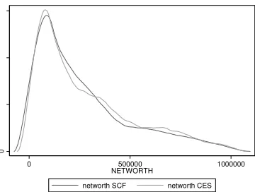
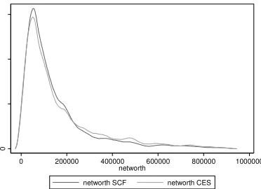
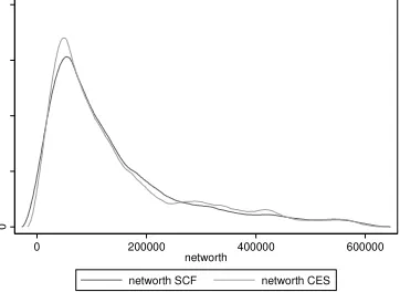
insert Figures 1-7 about here
Figures 1-7 report the graphs for household net wealth: we have chosen to report this variable because it includes both assets
and debt, and therefore summarizes better than other variables the results of the matching procedure. Although the two
distributions do not completely overlap because not all the SCF individuals are used as donors in the matching procedure, the
curves do show very similar patterns, again making sure that the matching procedure maintained the distributional properties of
the variables of interest.
We took these precautions because there are some conditions that have to be met in order not to commit errors when using
sample combination methods. First, the two different surveys must be two samples drawn from the same population. Second,
there must be a set of common variables on which to condition the matching procedure, as is clear from the above description of
the procedure. Third, the conditional independence assumption must hold. As for the first condition, both the CES and the SCF
are samples representing the US population. Their sample designs are different, since the SCF oversamples households that are
likely to be wealthier, while the CES does not. However, we decided to proceed with the sample combination procedure without
correcting for this difference, since any correction (that is, dropping a certain percentage of the wealthier SCF households)
would have involved a high degree of subjectivity. Despite this fact, the resulting dataset is robust to the alternative modus
operandi where the wealthiest SCF households are dropped before the sample combination. Actually, we also performed the
combination procedure after having got rid of the wealthiest households present in the SCF in order to get comparable income
distributions between the two surveys (in particular, dropping a percentage between 20 and 30% of the sample households with
the highest income depending on the survey year). The resulting dataset did not differ noticeably from the one that we used.
This is not surprising, because the Mahalanobis procedure discards the SCF households that differ considerably from the CES
households in terms of income (and age), so that most of the preliminarily dropped SCF individuals would have been discarded
anyway by the matching algorithm.
In terms of the second condition, there are many socio-demographic variables that are collected in both surveys, and the only
problem here is to recode the variables in order to have them expressed in the same way. This has been carried out making a
large use of the documentation that accompanies the public releases of the two surveys. Most recoding operations turned out to
be straightforward. The most interesting exception has been the recoding of the occupational sector variable for the 1989 and
1992 waves of the CES, where there is an additional category, "self-employed", which is not taken into account in the SCF. In
this case we performed a multinomial logit estimation to impute the occupational sector to the CES individuals labeled as
"self-employed" in order to proceed with the matching with the SCF. The estimation results were in line with the distributions of the
occupational variable both in the SCF and in the subsequent editions of the CES. As for the third condition, we must ensure that
we are not creating an artificial correlation between the consumption and the wealth variables by using the common
socio-demographic variables to perform the combination. Because of the exogenous nature of most of these variables, we believe that
9
3.3 The model
As a check of the relevance of the data handling process that we performed, we present the results of the estimation of an
econometric model close to the one used by BGP (2009).5
'
, 1 , 2 , 3 , 3 , , ,
log(
C
i t)
log(
Y
i t)
log(
fin
i t)
log(
house
i t)
log(
ore
i t)
Z
i t
i t, (1)where C is consumption (either non-durables or total consumption), Y is current income, fin is gross financial assets, house is the
value of the house of residence (if any), ore is the value of the rest of the housing/real estate assets.6 Finally, Z is a vector of
socio-demographic controls: age, educational level, a dummy for the marital status (married or with a partner/single), two
dummies for the race (one for African Americans, the other for non-Whites) and a dummy for the occupational status
(working/not working) of the household head; the number of persons in the household; a dummy for the homeownership status;
and three different dummies for the US geographical area (Northeast, Midwest and South, with West being the reference
region). As our dataset contains observations for households where the head is over 65 years old, we also include some
interaction terms to control for their different wealth and consumption dynamics of the old people. In particular, a dummy that
takes the value of 1 if the household head is over 65 years old is multiplied by income and by the relevant (according to the
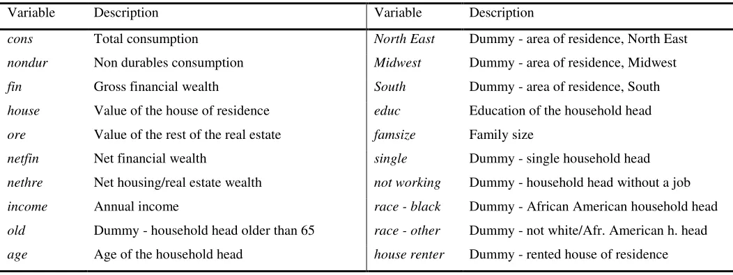
various model specifications, see below) wealth variables. Table 2 summarizes the variables used in the econometric analysis.
In order to investigate the importance of net compared to gross wealth we also estimate two additional specifications similar to
the one of equation (1): one in which financial wealth is diminished by total household debt (for the home-owners, this mainly
comprises mortgages), and one in which we use the value of the household housing/real estate assets (house + ore) diminished
by total household debt. The two net wealth variables are, respectively, netfin and nethre. Table 3 presents some descriptive
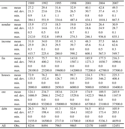
statistics of the consumption, income and wealth variables expressed in thousands of dollars to give an idea of the ranges and
average values of these important variables.
insert Table 3 about here
We estimate the models using two alternative dependent variables: the logarithm of total consumption and the logarithm of
non-durable goods expenditure. We disregard the expenditure on non-durable goods because its timing does not match the flow of
services coming from the goods. In particular, the relationship between consumption, income and wealth applies to the flow of
consumption, but durable goods expenditure “represents replacements and additions to a stock, rather than the service flow from
the existing stock” (Paiella 2007, 198). This may be one of the reasons why BGP (2009) find results that highly differ between
the specifications with total consumption and those with durables consumption. Therefore, we mainly concentrate on the results
for total and non durable goods consumption, showing that the use of the latter yields interesting additional insights.7
5 Similar models have also been used by Mehra (2001), Juster et al. (2004), and Paiella (2007b).
6 Note that we do not drop the households with wealth amounting to 0-0.99 dollars. Rather, we treat them as if their wealth amounts to 1 dollar, so that taking the logarithm yields a value of zero.
10
The models are estimated cross-sectionally (using data on 1989, 1992, 1995, 1998, 2001, 2004 and 2007) and by pooling data
over the seven surveys. In the latter case, year dummies are added as additional controls.
4. Results
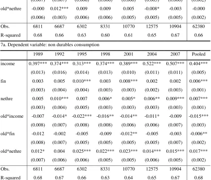
The results of the estimation of equation (1) are reported in tables 4 and 5 (with total and non durables consumption as the
dependent variable, respectively). CES sample weights have been used in all the estimates. The discussion below will highlight
the differences with the BGP (2009) results and will suggest some possible reasons behind them.
insert Tables 4 and 5 about here
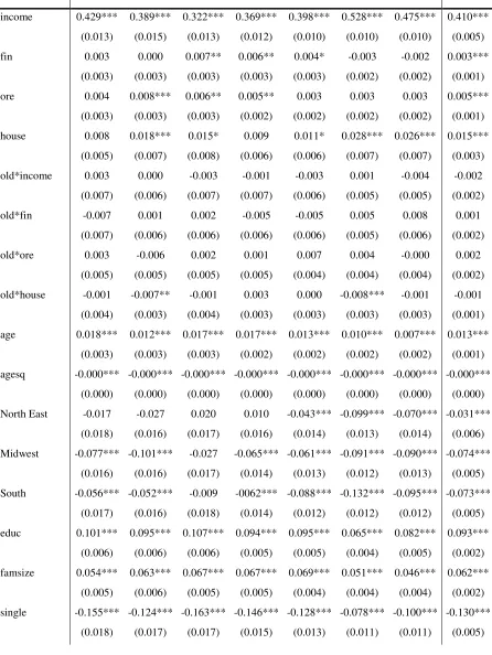
Current income plays a very important role in determining current consumption, with an estimated elasticity ranging between
.32 and .53, significantly higher than the BGP (2009) estimates and in line with estimates made using aggregate data (Duca et al.
2011). Turning to the wealth-related coefficients, different components have different effects on consumption. In particular,
gross financial wealth -fin- positively affected both types of consumption during the Nineties only (during the stock market
boom), while its estimated coefficients are not significantly different from zero for the rest of the sample period. However, when
significantly different from zero, the estimated elasticity of consumption to financial wealth is very low, being it close to .01,
less than half the point estimates of BGP (2009).
On the other hand, housing/real estate wealth positively affected consumption during the whole period of interest. In particular,
the estimated house of residence -house- elasticity is higher than the one related to the rest of real estate assets -ore- (with total
consumption as the dependent variable, the former lies between .01 and .03, while the latter never reaches .01). Even if the
magnitudes are once again different (and lower) than those estimated by BGP (2009), this result conforms to their findings.
Also, we confirm the downward trend of these elasticities up to 2001. In this respect, we are able to show a new result, due to
our longer time span. In particular, we find that the downward trend is reversed in 2004 and 2007, since the estimated elasticities
are considerably larger for these two periods. As in the case of the financial wealth coefficients of the Nineties, this does not
come as a complete surprise, because of the well known housing prices bubble that started in 2000 and abruptly ended with the
recent financial crisis in the second half of 2007. This suggests that housing/real estate wealth accounted for at least part of the
continued rise in consumption after the burst of the financial wealth bubble in 2001. It is also worth noting that these estimated
elasticities may be viewed as a lower bound for the actual wealth effects, since the model cannot take into account the increases
in consumption of the two years for which wealth has not been measured (since the SCF is a triennial survey), and also because
of the well-known underestimated consumption levels in the CES. The low estimated coefficients could also result from
measurement error issues leading to some kind of attenuation bias. However, the reassuring robustness checks on the
distributions of the wealth variables pre and post-sample combination lead us to believe that no attenuation bias is at work here.
As for the differences with BGP (2009), the reasons must lie either in the different sample combination procedure or in the
construction of the sample, or in both. The higher number of cells, the propensity score matching based on both income and age
11
roots of the different estimates.8 Finally, the larger number of observations and explanatory variables result in the larger portion
of the variability of consumption explained by our model. Our R squared ranges between .60 and .67, while in BGP (2009) it is
substantially lower, ranging between .34 and .43.
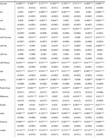
The behavior of the older households is investigated through the interaction terms between the “old” dummy and the income
and wealth variables. We see the inclusion of this set of controls as crucial, since both theory and previous empirical evidence
suggest that older households behave differently from younger ones (e.g. Miniaci et al. 2010). The estimates show that older
households experience a higher wealth effect from the value of the house of residence, reaching four cents per dollar of housing
wealth with non-durables consumption as the dependent variable. The pooled cross-section estimates confirm that consumption
patterns are sensitive to macroeconomic conditions, as all year dummies have highly significant coefficients.
Tables 6 and 7 report our estimates of the net wealth models, again for both dependent variables of interest.9 The number of
observations is lower than in the previous estimates due to the fact that we have to drop the households with negative net wealth
values (the net financial wealth specification has the lowest number of observations). It could also be expected that this
modification may bias the wealth coefficient, since only the richer households are considered in this part of the analysis. It is
hard to predict the direction of the bias, since richer households may be either more or less sensitive to the value of their wealth
when taking their consumption decisions.
insert Tables 6-7 about here
Table 6 (displaying the estimates of the net financial wealth specification) confirms the above findings for gross housing/real
estate wealth, while the results for the net financial wealth effects are less clear-cut. Most estimated coefficients for the net
financial wealth variable -netfin- are not statistically significant at standard levels (as in BGP, 2009). This is also the case when
non-durables consumption is used as the dependent variable (Table 6b). However, the pooled cross-section estimates suggest
that there is a small but positive net financial wealth effect. Similarly, in the model with net housing/real estate wealth -nethre-
(see Table 7) the estimated coefficients are lower than those associated to its gross measures. However, a non-negligible wealth
effect is estimated for the older households, as shown by the significance of the interaction term -old*nethre- (see Table 7b).
This confirms once again that the inclusion of older households permits a better understanding of consumption dynamics. All in
all, these results suggest the possibility of some myopia on the part of households, since consumption seems more sensitive to
gross wealth than net wealth (regardless of whether we calculate it out of financial or housing/real estate wealth).
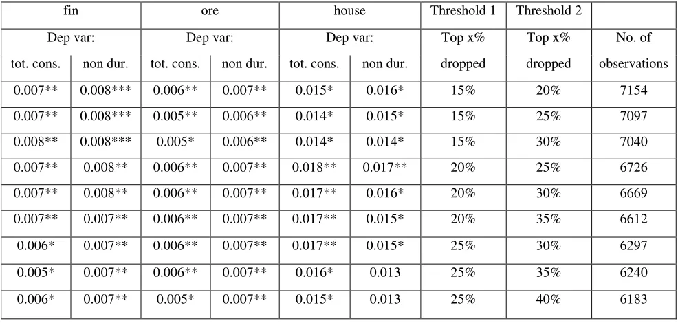
We investigated the robustness of our findings in several ways. Results hold when we restrict our sample to urban households
only (they are almost 90% of the sample). The same is true when we get rid of the 1% of household that are at the top and at the
bottom both of the income and of the consumption distributions. Results are also robust to several variations of the sample
combination procedure, as stated in the previous sections. One particular point deserves attention: using a high number of cells
should in principle lead to a more accurate sample combination, provided that small cells do not force matches of households
with extremely different values of income and age (i.e., relatively poor matches). The distance functions created during the
sample combination procedure allow us to identify the households that are poorly matched for removal. Table 8 reports the
8Actually, an additional reason may lie in the use of the CES sample weights that are not mentioned by BGP (2009).
12
estimated wealth coefficients (of the gross wealth model) when we drop households at the top of the distribution of the distance
variables using a number of different thresholds. While the first line displays the benchmark results, the rest of the Table reports
results for different values of the thresholds. Overall, the results are insensitive to the levels chosen. Table 8 presents evidence
for the 1995 data, but the same robustness is found for the rest of the data as well (not reported for the sake of brevity). This
robustness is not surprising, since our sample is very large, and it is unlikely that our results are driven by outliers or by small
subsamples of households.
5. Conclusions
In this article we investigate the role of wealth in household consumption during the period 1989-2007 using a household-level
cross-sectional dataset specifically built for this purpose. Following closely the rigorous guidelines on data matching outlined by
Ridder and Moffitt (2007), we adopt a sample combination procedure which differs considerably from that used earlier. We
combined US data from the CES and the SCF to get a series of cross-sections for the period 1989-2007 (in three years intervals).
In particular, the SCF was used as the donor survey: its wealth data were assigned to the CES households in order to build a
household-level dataset containing data for both consumption and wealth, as well as a substantial number of additional
socio-economic variables. This sample combination produced a large dataset (more than 70,000 observations) that preserved the
properties of the distributions of the variables of interest present in each of the two original surveys. We provide all the codes
that we used in order to perform the analysis (see the Web Appendix) in order to ensure its replication.
We performed an econometric exercise in order to assess the importance of the improved dataset construction procedures in
shaping the results of a wealth effect investigation, taking BGP (2009) as the reference point because they used a dataset derived
from the same two original surveys. By estimating a similar model, we showed that while some of the previous BGP (2009)
findings hold, most of them are considerably different. In particular, while we confirm that housing wealth effects are larger
than financial wealth effects, the quantitative importance of both types of effects is found to be substantially lower than
previously estimated (between .01 and .04 per dollar of housing/real estate wealth, even lower for financial wealth). We also
confirm a downward trend of the importance of wealth in determining consumption until 2001, but also document an inversion
of this tendency in 2004 and in 2007. Finally, the presence of households with head older than 65 years old in our sample
permits a better understanding of the wealth effect dynamics when net wealth is considered.
As for the implications of the estimated positive effects of wealth on consumption (ranging between 1 and 4 cents per dollar of
wealth), it would certainly be tempting to use our results to comment on the economic and financial crisis that originated from
the subprime mortgage market in 2007. However, we believe it to be impossible to extend our results to the interpretation of the
consumption and saving dynamics from the beginning of the crisis onwards, not only because our sample ends in 2007, but also
because it would be implausible to assume that wealth effects of the same magnitude are at work during both booms and
recessions. Indeed, some studies investigated the asymmetry of consumption responses to increases and decreases in wealth
(Shirvani and Wilbratte, 2000; Bertaut, 2002; Disney et al. 2002). The rationale behind the unequal wealth effects relates to the
assumption of diminishing marginal utility of wealth, where preferences are represented by convex utility functions (reflecting
13
consumers can readily reduce consumption in response to a wealth reduction, some consumers may find it difficult to borrow to
increase consumption. Thus, our analysis is unable to shed light on the mechanisms at work during the recent financial crisis.
This paper calls for further studies. Our findings highlight the importance of the type of wealth in shaping the link between
wealth and consumption. However, further and formal investigations on the nature of the wealth effects are needed to gain the
whole picture of the consumption-wealth nexus. Considering both the direct and indirect effects of wealth on consumption
would render a more complete understanding of the phenomenon.
References
Aguiar, M. & Hurst, E. (2005). Consumption vs. expenditure. Journal of Political Economy 113(5), 919-948.
Aguiar, M. & Hurst, E. (2007). Lifecycle prices and production. American Economic Review 97(5), 1533-1559.
Ando, A., & Modigliani, F. (1963). The “life cycle” hypothesis of saving: aggregate implications and tests. American Economic
Review, 53(1), 55-84.
Attanasio, O., & Banks, J. (2001). The assessment: household saving - issues in theory and policy. Oxford Review of Economic
Policy, 17(1), 1-19.
Attanasio, O., & Weber, G. (2010). Consumption and saving: Models of intertemporal allocation and their implications for
public policy. Journal of Economic Literature 48(3), 693-751.
Becker, G. (1965). A theory of the allocation of time. The Economic Journal, 75, 493-517.
Becker, G. (1981). A treatise on the family. Harvard University Press: Cambridge.
Belski, E., & Prakken, J. (2004). Housing wealth effects: housing’s impact on wealth accumulation, wealth distribution and
consumer spending. Harvard University, Joint Center for Housing Studies, W04-13.
Benjamin, J.D., Chinloy, P., & Jud, G.D. (2004). Real estate versus financial wealth in consumption. Journal of Real Estate
Finance and Economics, 29(3), 341-354.
Bertaut, C.C. (2002). Equity prices, household wealth, and consumption growth in foreign industrial countries: wealth effects in
the 1990s. International Finance Discussion Papers 724, Board of Governors of the Federal Reserve System.
Bostic, R., Gabriel, S., & Painter, G. (2009). Housing wealth, financial wealth, and consumption: new evidence from micro data.
Regional Science and Urban Economics, 39, 79-89.
Browning, M.J., Deaton, A.S., & Irish, M. (1985). A profitable approach to labor supply and commodity demands over the
life-cycle. Econometrica, 53, 503-544.
Campbell, J.Y., & Cocco, J.F. (2007). How do house prices affect consumption? Evidence from micro data. Journal of
Monetary Economics, 54, 591-621.
Carroll, C., Dynan, K. & Krane, S. (2003). Unemployment risk and precautionary wealth: Evidence from households’ balance
sheets. Review of Economics and Statistics 85, 586-604.
Carroll, C., Otsuka, M., & Slacalek, J. (2006). How large is the houseing wealth effect? A new approach. NBER Working Paper
14
Case, K., & Quigley, J. (2008). How housing booms unwind: income effects, wealth effects, and feedbacks through financial
markets. Journal of Housing Policy, 8(2), 161-180.
Case, K., Quigley, J., & Shiller, R. (2005). Comparing wealth effects: the stock market versus the housing market. Advances in
Macroeconomics, Vol. 5(1), 1-32.
Catte, P., Girouard, N., Price, R., & André, C. (2004). Housing markets, wealth and the business cycle. OECD Economics
Department Working Paper 394.
Davis, M., & Palumbo, M. (2001). A primer on the economics and time series econometrics of wealth effects. Board of
Governors of the Federal Reserve System, Finance and Economics Discussion Paper Series 2001-09, Washington DC.
Deaton, A.S. (1985). Panel data from times series of cross-sections. Journal of Econometrics, 30, 109-126.
D'Orazio, M., Di Zio, M., & Scanu, M. (2006). Statistical matching: theory and practice. Chichester, England: Wiley.
Del Boca, D., Locatelli, & M., Vuri, D. (2005). Child care choices of Italian households. Review of Economics of the
Household, 3, 453-477.
Disney, R., Henley, A., & Jevons, D. (2002). House price shocks, negative equity and household consumption in the UK in the
1990s. Royal Economic Society Annual Conference.
Dvornak, N., & Kohler, M. (2007). Housing wealth, stock market wealth and consumption: a panel analysis for Australia.
Economic Record, 83(261), 117-130.
Dynan, K., & Maki, D. (2001). Does stock market wealth matter for consumption? Finance and Economics Discussion Series
2001:23, Washington Board of Governors of the Federal Reserve System.
Duca, J.V., Muellbauer, J., & Murphy, A. (2011). Credit market architecture and the boom and bust in US consumption. Mimeo.
Edison, H., & Sløk, T. (2002). Stock market wealth effects and the new economy: a cross-country study. International Finance
5(1), 1-22.
Engelhardt, G.V. (1996). Consumption, down payments, and liquidity constraints. Journal of Money, Credit and Banking, 28(2),
255-271.
Fernandez-Villaverde, J., & Krueger, D. (2007). Consumption over the life-cycle: facts from Consumer Expenditure Survey.
The Review of Economics and Statistics, 89(3), 552-565.
Garner, T., Janini, G., Passero, W., Paszkiewicz, L., & Vendemia, M. (2006). The CE and the PCE: a comparison. Monthly
Labor Review, September, 20-46.
Ghez, G. & Becker, G. (1975). The allocation of time and goods over the life cycle. Columbia University Press, New York.
Greenspan, A. (2003). Remarks at the annual convention of the Independent Community Bankers of America, Orlando,
Florida,” March 4th
.
Hurst, E., & Stafford, F. (2004). Home is where the equity is: Mortgage refinancing and household consumption. Journal of
Money, Credit and Banking, 36(6), 985-1014.
Juster, T., Lupton, J., Smith, J., & Stafford, F. (2005). The decline in household saving and the wealth effect. The Review of
Economics and Statistics, 87(4), 20-27.
Kennickell, A. (1998). Multiple Imputation in the Survey of Consumer Finances.
15
Lehnert, A. (2004). Housing, consumption and credit constraints. Finance and Economics Discussion Series, Board of
Governors of the Federal Reserve System.
Lettau, M., & Ludvigson, S. (2004). Understanding trend and cycle in asset values: reevaluating the wealth effect on
consumption. American Economic Review, 94(1), 279-299.
Levin, L. (1998). Are assets fungible? Testing the behavioral theory of life-cycle savings. Journal of Economic Behavior and
Organization, 36, 59-83.
Ludvigson, S., & Steindel, C. (1999). How important is the stock market effect on consumption? Federal Reserve Bank of New
York Economic Policy Review, July.
Maki, D.M., & Palumbo, M.G. (2001). Disentangling the wealth effect: a cohort analysis of household saving in the 1990s.
Finance and Economics Discussion Series, Board of Governors of the Federal Reserve System.
Mehra, Y.P. (2001). The wealth effect in empirical life-cycle aggregate consumption equations. Federal Reserve Bank of
Richmond Economic Quarterly 87/2.
Miniaci, R., Monfardini, C., & Weber, G. (2010). How does consumption change upon retirement? Empirical Economics, 38,
257-280.
Montalto, C., & Sung, J. (1996). Multiple imputation in the 1992 Survey of Consumer Finances. Financial Counseling and
Planning, 7.
Morris, E.D. (2006). Examining the wealth effect from home price appreciation. University of Michigan, mimeo.
Paiella, M. (2009). The stock market, housing and consumer spending: a survey of the evidence on wealth effect. Journal of
Economic Surveys, 23(5), 947-973.
Paiella, M. (2007). Does wealth affect consumption? Evidence for Italy. Journal of Macroeconomics, 29, 189-205.
Parker, J.A. (1999). Spendthrift in America? On two decades of decline in the US saving rate. NBER Macroeconomics Annual,
14, 317-370.
Poterba, J.M. (2000). Stock market wealth and consumption. The Journal of Economic Perspectives, 14(2), 99-118.
Ridder, G., & Moffitt, R. (2007). The econometrics of data combination. Handbook of Econometrics, 6, 5469-5547.
Rosati, N. (1998). Matching statistico tra dati ISTAT sui consumi e dati Bankitalia sui redditi per il 1995. Padova Economics
Department Discussion Paper, 7.
Rubin, D.B. (1987). Multiple imputation for nonresponse in surveys. New York: Wiley.
Shirvani, H., & Wilbratte, B. (2000). Does consumption respond more strongly to stock market declines than to increases?
International Economic Journal, 14(3), 41-49.
16
[image:17.612.63.243.121.257.2]Figures
Figure 1: Household net wealth kernel distribution, 2007
0
0 500000 1000000
NETWORTH
[image:17.612.62.245.327.460.2]networth SCF networth CES
Figure 2: Household net wealth kernel distribution, 2004
0
0 200000 400000 600000 800000 1000000
NETWORTH
[image:17.612.62.243.527.662.2]networth SCF networth CES
Figure 3: Household net wealth kernel distribution, 2001
0
0 200000 400000 600000 800000 1000000
networth
17
Figure 4: Household net wealth kernel distribution, 1998
0
0 200000 400000 600000 800000 1000000
networth
[image:18.612.63.244.290.425.2]networth SCF networth CES
Figure 5: Household net wealth kernel distribution, 1995
0
0 200000 400000 600000 800000 1000000
networth
networth SCF networth CES
Figure 6: Household net wealth kernel distribution, 1992
0
0 200000 400000 600000 800000 1000000
networth
[image:18.612.62.248.490.625.2]18
Figure 7: Household net wealth kernel distribution, 1989
0
0 200000 400000 600000
networth
19
[image:20.612.42.532.115.289.2]Tables
Table 1. Correlations between logarithmic income and the wealth (SCF) variables
2007 2004 2001 1998
SCF CES SCF CES SCF CES SCF CES
fin 0.26** 0.16** 0.26** 0.18** 0.27** 0.14** 0.22** 0.11* hre 0.27** 0.30** 0.25** 0.26** 0.24** 0.18** 0.19** 0.17** asset 0.32** 0.29** 0.30** 0.26** 0.31** 0.20** 0.25** 0.17** debt 0.46** 0.43** 0.41** 0.40** 0.47** 0.42** 0.38** 0.29** networth 0.30** 0.26** 0.28** 0.23** 0.29** 0.18** 0.23** 0.16**
1995 1992 1989
SCF CES SCF CES SCF CES
fin 0.18** 0.12* 0.24** 0.19** 0.25** 0.08**
hre 0.20** 0.09* 0.16** 0.09** 0.21** 0.10**
asset 0.24** 0.12** 0.21** 0.11** 0.27** 0.13** debt 0.32** 0.29** 0.28** 0.14** 0.39** 0.33** networth 0.22** 0.10** 0.19** 0.10** 0.25** 0.12**
Notes: fin (gross financial wealth), hre (housing/real estate wealth), asset (financial + housing/real estate wealth), debt
[image:20.612.43.569.370.568.2](household debt), networth (asset - debt). *, ** significant at 5 and 1% respectively.
Table 2. List of variables used in the regressions
Variable Description Variable Description
cons Total consumption North East Dummy - area of residence, North East
nondur Non durables consumption Midwest Dummy - area of residence, Midwest
fin Gross financial wealth South Dummy - area of residence, South
house Value of the house of residence educ Education of the household head
ore Value of the rest of the real estate famsize Family size
netfin Net financial wealth single Dummy - single household head
nethre Net housing/real estate wealth not working Dummy - household head without a job
income Annual income race - black Dummy - African American household head
old Dummy - household head older than 65 race - other Dummy - not white/Afr. American h. head
20
Table 3. Descriptive statistics of consumption, income and wealth variables (thousands of $)
1989 1992 1995 1998 2001 2004 2007
cons mean 27.2 29.4 31.6 32.9 40.1 42.8 49.5
std. dev. 21.3 23.6 23.6 26.5 30.7 37.4 41.3
min. 0.9 1.4 1.1 0.7 0.8 0.0 0.1
max. 384.1 551.9 334.6 487.4 434.1 1018.1 867.5
nondur mean 15.9 17.5 18.5 19.0 24.0 26.4 30.9
std. dev. 12.3 14.6 13.4 15.0 18.6 24.9 28.7
min. 0.5 0.5 0.8 0.7 0.1 0.0 0.1
max. 212.0 532.8 149.8 274.3 246.1 936.8 835.1
income mean 31.0 34.0 35.9 41.3 48.3 57.5 66.6
std. dev. 25.9 28.3 29.5 39.7 45.6 51.4 62.6
min. 0.3 0.1 0.0 0.0 0.0 0.5 0.3
max. 415.7 225.4 280.0 590.2 600.1 567.5 549.7
fin mean 83.5 75.7 91.3 143.0 185.9 177.5 216.3
std. dev. 795.8 400.2 519.1 1587.1 1271.3 1030.7 1090.6
min. 0.0 0.0 0.0 0.0 0.0 0.0 0.0
max. 28100.0 25200.0 19600.0 142000.0 77200.0 42700.0 37500.0
houses mean 72.9 76.2 80.3 99.7 124.3 179.1 225.3
std. dev. 135.5 152.4 126.7 191.5 235.0 346.2 408.4
min. 0.0 0.0 0.0 0.0 0.0 0.0 0.0
max. 2000.0 6000.0 2850.0 6000.0 5000.0 10500.0 10400.0
ore mean 124.1 234.7 183.6 212.9 174.9 189.5 245.9
std. dev. 1686.9 2866.1 2342.2 1529.6 1422.5 966.8 1167.9
min. 0.0 0.0 0.0 0.0 0.0 0.0 0.0
max. 92400.0 93200.0 150000.0 50200.0 65700.0 23100.0 37500.0
debt mean 26.3 38.5 41.3 52.9 54.5 85.0 105.9
std. dev. 67.7 198.4 103.1 164.1 102.0 173.4 205.1
min. 0.0 0.0 0.0 0.0 0.0 0.0 0.0
max. 3155.0 16500.0 2717.0 11700.0 1830.0 5336.3 4659.0
All Obs. 8216 8494 7963 9865 12170 14405 12451
21
Table 4. Equation (2), dependent variable: total consumption
1989 1992 1995 1998 2001 2004 2007 Pooled
income 0.429*** 0.389*** 0.322*** 0.369*** 0.398*** 0.528*** 0.475*** 0.410***
(0.013) (0.015) (0.013) (0.012) (0.010) (0.010) (0.010) (0.005)
fin 0.003 0.000 0.007** 0.006** 0.004* -0.003 -0.002 0.003***
(0.003) (0.003) (0.003) (0.003) (0.003) (0.002) (0.002) (0.001)
ore 0.004 0.008*** 0.006** 0.005** 0.003 0.003 0.003 0.005***
(0.003) (0.003) (0.003) (0.002) (0.002) (0.002) (0.002) (0.001)
house 0.008 0.018*** 0.015* 0.009 0.011* 0.028*** 0.026*** 0.015***
(0.005) (0.007) (0.008) (0.006) (0.006) (0.007) (0.007) (0.003)
old*income 0.003 0.000 -0.003 -0.001 -0.003 0.001 -0.004 -0.002
(0.007) (0.006) (0.007) (0.007) (0.006) (0.005) (0.005) (0.002)
old*fin -0.007 0.001 0.002 -0.005 -0.005 0.005 0.008 0.001
(0.007) (0.006) (0.006) (0.006) (0.006) (0.005) (0.006) (0.002)
old*ore 0.003 -0.006 0.002 0.001 0.007 0.004 -0.000 0.002
(0.005) (0.005) (0.005) (0.005) (0.004) (0.004) (0.004) (0.002)
old*house -0.001 -0.007** -0.001 0.003 0.000 -0.008*** -0.001 -0.001
(0.004) (0.003) (0.004) (0.003) (0.003) (0.003) (0.003) (0.001)
age 0.018*** 0.012*** 0.017*** 0.017*** 0.013*** 0.010*** 0.007*** 0.013***
(0.003) (0.003) (0.003) (0.002) (0.002) (0.002) (0.002) (0.001)
agesq -0.000*** -0.000*** -0.000*** -0.000*** -0.000*** -0.000*** -0.000*** -0.000***
(0.000) (0.000) (0.000) (0.000) (0.000) (0.000) (0.000) (0.000)
North East -0.017 -0.027 0.020 0.010 -0.043*** -0.099*** -0.070*** -0.031***
(0.018) (0.016) (0.017) (0.016) (0.014) (0.013) (0.014) (0.006)
Midwest -0.077*** -0.101*** -0.027 -0.065*** -0.061*** -0.091*** -0.090*** -0.074***
(0.016) (0.016) (0.017) (0.014) (0.013) (0.012) (0.013) (0.005)
South -0.056*** -0.052*** -0.009 -0062*** -0.088*** -0.132*** -0.095*** -0.073***
(0.017) (0.016) (0.018) (0.014) (0.012) (0.012) (0.012) (0.005)
educ 0.101*** 0.095*** 0.107*** 0.094*** 0.095*** 0.065*** 0.082*** 0.093***
(0.006) (0.006) (0.006) (0.005) (0.005) (0.004) (0.005) (0.002)
famsize 0.054*** 0.063*** 0.067*** 0.067*** 0.069*** 0.051*** 0.046*** 0.062***
(0.005) (0.006) (0.005) (0.005) (0.004) (0.004) (0.004) (0.002)
single -0.155*** -0.124*** -0.163*** -0.146*** -0.128*** -0.078*** -0.100*** -0.130***
22
not working -0.105*** -0.113*** -0.085*** -0.083*** -0.034** -0.011 -0.001 -0.061***
(0.021) (0.022) (0.022) (0.018) (0.016) (0.016) (0.014) (0.007)
race-black -0.103*** -0.087*** -0.054** -0.057*** -0.061*** -0.053*** -0.070*** -0.067***
(0.024) (0.022) (0.022) (0.019) (0.017) (0.015) (0.016) (0.007)
race-other -0.054 -0.0312 -0.062* -0.036 -0.021 -0.020 -0.029 -0.031***
(0.042) (0.037) (0.036) (0.032) (0.027) (0.022) (0.024) (0.011)
home renter 0.027 0.082 0.052 0.037 0.014 0.269*** 0.231*** 0.087***
(0.061) (0.074) (0.091) (0.073) (0.069) (0.081) (0.086) (0.030)
constant 4.952*** 5.428*** 6.018*** 5.586*** 5.524*** 4.117*** 4.861*** 5.177***
(0.131) (0.150) (0.151) (0.118) (0.115) (0.113) (0.113) (0.050)
y1992 0.049***
(0.008)
y1995 0.105***
(0.008)
y1998 0.068***
(0.008)
y2001 0.171***
(0.008)
y2004 0.125***
(0.008)
y2007 0.238***
(0.008)
Obs. 7322 7596 7154 9865 12170 14405 12387 70899
R-squared 0.67 0.66 0.63 0.60 0.60 0.64 0.65 0.65
Notes: All the estimations were carried out using the Repeated Imputation Inference (RII) using all the five implications
resulting from the SCF procedure of imputing missing income values. CES sample weights have been used. Standard errors in
23
Table 5. Equation (2), dependent variable: non durables consumption
1989 1992 1995 1998 2001 2004 2007 Pooled
income 0.400*** 0.368*** 0.317*** 0.366*** 0.393*** 0.513*** 0.488*** 0.400***
(0.013) (0.014) (0.013) (0.011) (0.009) (0.011) (0.010) (0.005)
fin 0.003 0.007** 0.008*** 0.005** 0.007*** 0.001 0.003 0.006***
(0.003) (0.003) (0.003) (0.002) (0.002) (0.002) (0.002) (0.001)
ore 0.005 0.006** 0.007** 0.004** 0.002 0.003 0.004** 0.004***
(0.003) (0.003) (0.003) (0.002) (0.002) (0.002) (0.002) (0.001)
house 0.012** 0.014** 0.016* 0.014** 0.013** 0.029*** 0.025*** 0.019***
(0.005) (0.006) (0.008) (0.006) (0.006) (0.006) (0.007) (0.001)
old*income -0.006 -0.014** -0.014** -0.012* -0.010* -0.008 -0.012** -0.012***
(0.007) (0.007) (0.007) (0.007) (0.006) (0.005) (0.006) (0.003)
old*fin -0.015** -0.005 -0.002 -0.010* -0.12** -0.008* -0.004 -0.008***
(0.007) (0.007) (0.006) (0.005) (0.006) (0.005) (0.007) (0002)
old*ore 0.000 -0.008 -0.001 0.001 0.006 0.003 0.002 0.001
(0.006) (0.005) (0.005) (0.005) (0.004) (0.004) (0.004) (0.002)
old*house 0.016*** 0.016*** 0.017*** 0.020*** 0.017*** 0.013*** 0.017*** 0.017***
(0.004) (0.004) (0.004) (0.003) (0.003) (0.003) (0.003) (0.001)
age 0.013*** 0.012*** 0.014*** 0.013*** 0.011*** 0.005** 0.005*** 0.011***
(0.003) (0.003) (0.003) (0.002) (0.002) (0.002) (0.002) (0.001)
agesq -0.000*** -0.000*** -0.000*** -0.000*** -0.000*** -0.000 -0.000** -0.000***
(0.000) (0.000) (0.000) (0.000) (0.000) (0.000) (0.000) (0.000)
North East 0.045*** 0.046*** 0.075*** 0.052*** -0.029** -0.069*** -0.047*** 0.011*
(0.017) (0.017) (0.017) (0015) (0.014) (0.013) (0.014) (0.006)
Midwest -0.023 -0.031*** 0.051*** 0.005 -0.020 -0.039*** -0.018 -0.011**
(0.015) (0.016) (0.017) (0.013) (0.013) (0.012) (0.013) (0.005)
South 0.000 0.010 0.052*** 0.010 -0.058*** -0.082*** -0.032*** -0.017***
(0.015) (0.016) (0.017) (0.013) (0.012) (0.012) (0.012) (0.005)
educ 0.093*** 0.089*** 0.102*** 0.088*** 0.098*** 0.068*** 0.080*** 0.089***
(0.006) (0.006) (0.006) (0.005) (0.005) (0.004) (0.005) (0.002)
famsize 0.069*** 0.075*** 0.077*** 0.074*** 0.067*** 0.055*** 0.044*** 0.068***
(0.005) (0.005) (0.005) (0.004) (0.004) (0.004) (0.004) (0.002)
single -0.141*** -0.128*** -0.143*** -0.123*** -0.131*** -0.105*** -0.114*** -0.130***
24
not working -0.099*** -0.100*** -0.095*** -0.085*** -0.040** -0.028* -0.016 -0.066***
(0.020) (0.021) (0.022) (0.018) (0.016) (0.016) (0.014) (0.007)
race-black -0.073*** -0.046** -0.022 -0.054*** -0.050*** -0.058*** -0.064*** -0.051***
(0.023) (0.022) (0.021) (0.017) (0.016) (0.015) (0.016) (0.007)
race-other -0.075* -0.036 -0.037 -0.032 -0.060** -0.050** -0.076*** -0.050***
(0.044) (0.046) (0.035) (0.033) (0.027) (0.021) (0.024) (0.011)
home renter 0.036 0.024 0.024 0.048 0.009 0.235*** 0.205** 0.095***
(0.057) (0.062) (0.093) (0.065) (0.065) (0.073) (0.085) (0.027)
constant 4.679*** 5.023*** 5.475*** 5.059*** 4.987*** 3.768*** 4.142*** 4.670***
(0.125) (0.139) (0.145) (0.112) (0.106) (0.110) (0.117) (0.047)
y1992 0.057***
(0.008)
y1995 0.097***
(0.007)
y1998 0.056***
(0.007)
y2001 0.181***
(0.007)
y2004 0.148***
(0.007)
y2007 0.258***
(0.007)
Obs. 7322 7596 7154 9865 12170 14405 12387 70899
R-squared 0.68 0.67 0.65 0.63 0.63 0.65 0.65 0.67
Notes: All the estimations were carried out using the Repeated Imputation Inference (RII) using all the five implications
resulting from the SCF procedure of imputing missing income values. CES sample weights have been used. Standard errors in
25
Table 6. Equation (3), two different dependent variables
6a. Dependent variable: total consumption
1989 1992 1995 1998 2001 2004 2007 Pooled
income 0.431*** 0.375*** 0.296*** 0.365*** 0.392*** 0.502*** 0.485*** 0.398***
(0.016) (0.022) (0.018) (0.017) (0.013) (0.014) (0.013) (0.007)
netfin 0.002 0.004 0.008 0.005 0.009** -0.007* -0.001 0.004***
(0.004) (0.005) (0.005) (0.003) (0.004) (0.004) (0.003) (0.001)
ore 0.004* 0.007* 0.006 0.004 0.004 0.004 0.000 0.005***
(0.003) (0.004) (0.004) (0.003) (0.003) (0.003) (0.003) (0.001)
house 0.016** 0.018 0.008 0.018** 0.010 0.045*** 0.030*** 0.020***
(0.008) (0.013) (0.012) (0.009) (0.007) (0.010) (0.010) (0.003)
old*income 0.003 -0.002 0.003 0.000 0.001 0.006 0.002 0.000
(0.009) (0.007) (0.009) (0.008) (0.008) (0.006) (0.007) (0.003)
old*netfin -0.004 0.002 0.002 -0.006 -0.010 0.004 0.004 -0.000
(0.009) (0.008) (0.008) (0.006) (0.008) (0.006) (0.007) (0.003)
old*ore -0.000 -0.008 -0.001 0.005 0.007 0.003 0.003 0.002
(0.006) (0.006) (0.006) (0.006) (0.005) (0.005) (0.005) (0.002)
old*house -0.002 -0.007* -0.002 0.002 0.002 -0.011*** -0.004 -0.003*
(0.004) (0.004) (0.004) (0.004) (0.003) (0.003) (0.004) (0.001)
Obs. 4491 4268 3982 5555 7091 7360 6495 39242
R-squared 0.68 0.67 0.64 0.61 0.62 0.65 0.69 0.67
6b. Dependent variable: non durables consumption
1989 1992 1995 1998 2001 2004 2007 Pooled
income 0.393*** 0.363*** 0.285*** 0.365*** 0.386*** 0.483*** 0.494*** 0.386***
(0.016) (0.021) (0.018) (0.017) (0.012) (0.015) (0.014) (0.007)
netfin 0.002 0.007 0.007 0.004 0.006* -0.002 0.004 0.005***
(0.005) (0.005) (0.005) (0.003) (0.004) (0.004) (0.003) (0.001)
ore 0.003 0.005 0.008** 0.004 0.004 0.005 0.002 0.005***
(0.003) (0.004) (0.004) (0.003) (0.003) (0.003) (0.003) (0.001)
house 0.020*** 0.014 0.008 0.023*** 0.015** 0.045*** 0.028*** 0.025***
(0.007) (0.012) (0.012) (0.008) (0.007) (0.009) (0.010) (0.003)
old*income -0.002 -0.013 -0.006 -0.006 -0.006 0.003 0.001 -0.006*
(0.010) (0.008) (0.009) (0.008) (0.007) (0.006) (0.009) (0.003)
26
(0.012) (0.009) (0.008) (0.006) (0.007) (0.006) (0.008) (0.003)
old*ore -0.002 -0.009 -0.006 0.002 0.004 0.002 0.004 -0.000
(0.007) (0.006) (0.007) (0.006) (0.005) (0.005) (0.004) (0.002)
old*house 0.013*** 0.011*** 0.013*** 0.017*** 0.016*** 0.007* 0.011*** 0.013***
(0.004) (0.004) (0.005) (0.004) (0.003) (0.004) (0.004) (0.002)
Obs. 4491 4268 3982 5555 7091 7360 6495 39242
R-squared 0.68 0.67 0.65 0.64 0.64 0.65 0.68 0.67
Notes: All the estimations were carried out using the Repeated Imputation Inference (RII) using all the five implications
resulting from the SCF procedure of imputing missing income values. CES sample weights have been used. Standard errors in