arXiv:hep-th/0609157v1 22 Sep 2006
Preprint typeset in JHEP style - HYPER VERSION AEI-2006-071 HU-EP-06/31 ITP-UU-06-39 SPIN-06-33 TCDMATH 06-13
The Off-shell Symmetry Algebra of the
Light-cone
AdS
5
×
S
5
Superstring
Gleb Arutyunova∗†, Sergey Frolovb†, Jan Plefkac and Marija Zamaklard a Institute for Theoretical Physics and Spinoza Institute,
Utrecht University, 3508 TD Utrecht, The Netherlands
b School of Mathematics, Trinity College, Dublin 2, Ireland c Humboldt-Universit¨at zu Berlin, Institut f¨ur Physik,
Newtonstraße 15, D-12489 Berlin, Germany
d Max-Planck-Institut f¨ur Gravitationsphysik, Albert-Einstein-Institut
Am M¨uhlenberg 1, D-14476 Potsdam, Germany
Abstract:We analyze thepsu(2,2|4) supersymmetry algebra of a superstring
prop-agating in the AdS5×S5 background in the uniform light-cone gauge. We consider
the off-shell theory by relaxing the level-matching condition and take the limit of infinite light-cone momentum, which decompactifies the string world-sheet. We fo-cus on the psu(2|2)⊕psu(2|2) subalgebra which leaves the light-cone Hamiltonian invariant and show that it undergoes extension by a central element which is ex-pressed in terms of the level-matching operator. This result is in agreement with the conjectured symmetry algebra of the dynamic S-matrix in the dualN = 4 gauge theory.
Contents
1. Introduction 1
2. Gauged-fixed string sigma-model 4
3. Symmetry generators in the light-cone gauge 7
3.1 General structure of the symmetry generators 7 3.2 Moment map and the Poisson brackets 9
3.3 Explicit basis 12
4. Deriving the central charges 13
5. Concluding remarks 17
6. Appendix 18
6.1 The gauge-fixed Hamiltonian 18
6.2 Symmetry generators 20
6.3 Covariant notation 21
6.4 The explicit form of the su(2|2)R generators 23
6.5 The su(2|2)R supercharge at quartic field order 24
6.6 The explicit form of the su(2|2)L generators 24
6.7 The centrality of the level-matching and Hamiltonian 26
1. Introduction
Understanding the symmetries of physical systems usually leads to the most elegant way of solving them. The Green-Schwarz string theory on the AdS5×S5 background
[1] presents a prime example of a system with a very large number of symmetries. The manifest global symmetry of the string sigma-model is given by the PSU(2,2|4) super-group, an isometry group of the target coset space. Moreover the world-sheet theory is a classically integrable model [2], possessing thus an infinite number of (non)local integrals of motion. Finally, being a superstring theory, it possesses the local gauge symmetries of world-sheet diffeomorphisms and the fermionic κ-symmetry.
Nevertheless, the quantisation of the superstring on AdS5 ×S5 in a covariant
and allows one to invoke the notion of asymptotic states and the machinery of the string S-matrix [3, 4, 5]. Based on extensive work [6]-[11] it is becoming more and more apparent that a particularly convenient world-sheet gauge choice is the so-called
generalised uniform light-cone gauge [8, 10]. World-sheet excitations in this gauge are closely related to the spin chain excitation picture appearing on the gauge theory side, and thus make the link between the two more transparent. Also, similarly as in flat space, this is the only gauge which makes the Green-Schwarz fermions tractable.
The generalised uniform light-cone gauge, however, has the unpleasant feature that the gauge-fixed action does not possess world-sheet Lorentz invariance. The fact that this symmetry is absent makes the construction of the world-sheet S-matrix particularly involved: standard constraints on the form of S-matrix arising from the requirement of Lorentz invariance cannot be directly implemented, but require subtle constructions [12, 13]. It is thus extremely important to understand the symmetries of the world-sheet theory in this gauge, how they constrain the form of the S-matrix, and how they are connected with the symmetries present in the gauge theory.
The generators of the superisometry algebrapsu(2,2|4) of the string sigma-model can be split into two groups: those which (Poisson) commute with the Hamiltonian and those which do not. The former comprise the su(2|2)⊕su(2|2) subalgebra of the full psu(2,2|4) algebra, sharing the same central element which corresponds to the Hamiltonian. Another separation of the psu(2,2|4) generators is into dynamical and kinematical generators, depending on whether they do or do not depend on the unphysical field x−.
There are three important facts related to the presence of the unphysical field
x− in the light-cone world-sheet theory. One is that when solved in terms of physical fields, x− is a non-local expression. Second is that the zero mode of the field x− is a priori non-zero and has a non-trivial Poisson bracket with the total light-cone mo-mentum P+. This implies that dynamical charges change the light-cone momentum P+. It also follows, that the zero mode part of the operatoreiαx− plays precisely the
role of a “length changing” operator, given that in the uniform light cone gauge, the total light cone momentum P+ is naturally identified with the circumference of the
world-sheet cylinder. However, and this shall be exploited extensively in the present paper, in the limit of infinite light-cone momentum P+, the fluctuations of the P+
are irrelevant, and the zero mode of x− can be thus consistently ignored. Thirdly, the differentiated field x′
− is a density of the world-sheet momentum related to the
presence of rigid symmetries in the space-like σ-direction of the light-cone gauge fixed string action. In the case of closed strings, the periodicity of fields implies that the total world-sheet momentum pws has to vanish. This constraint is called the
level-matching condition.
world-sheet S-matrix, one needs to: (a) relax the level-matching condition and (b) consider the limit P+ → ∞. If level-matching is not satisfied, we will refer to
the theory as “off-shell”. The limit (b) is necessary in order to define asymptotic states and it basically defines the gauge fixed world-sheet theory on the plane, rather than on a cylinder of circumference P+ [14]-[20]. In this paper, we will restrict the
consideration to this limit, only briefly commenting on the finite P+ configurations
in the discussion.
If the level-matching condition holds, the su(2|2)⊕su(2|2) subalgebra of the
psu(2,2|4) algebra is spanned by those generators which commute with the world-sheet Hamiltonian. Giving up the level-matching condition in string theory in prin-ciple could spoil the on-shell psu(2,2|4) symmetry algebra of the world-sheet theory and in particular the centrality of the Hamiltonian with respect to the su(2|2)⊕
su(2|2) subalgebra. The main goal of this paper is the derivation of the string world-sheet symmetry algebra in the case when the level-matching is relaxed.
In N = 4 gauge theory the analogue of the level-matching condition is im-plemented by considering gauge-invariant operators, i.e. traces of products of fields. Hence relaxing the level-matching in string theory corresponds to “opening” the trace of fields in gauge theory, i.e considering open rather than closed spin chains. Beisert has argued in [5] that opening the traces in gauge theory (and considering infinitely long operators) leads to a modification of the su(2|2)⊕su(2|2) algebra: the algebra receives two central charges in addition to the Hamiltonian, which are functions of the momentum carried by the one-particle excitations. The Hamiltonian remains a central element. This centrally extended symmetry algebra beautifully allowed for the derivation of the dispersion relation of the elementary “magnon” excitations as well as for the restriction of the form of S-matrix down to one unknown function.
The main result of this paper is thederivationof the centrally extendedsu(2|2)⊕
su(2|2) algebra in string theory both at the classical and quantum level. By explicit computations, we show that relaxing the level-matching condition in string theory in the limit of infinite light-cone momentum necessarily leads to an enlargement of the su(2|2)⊕su(2|2) algebra by a common central element which is proportional to the level-matching condition. In addition, the Hamiltonian remains central, as it was the case for the on-shell algebra.
the dynamical charges depend on the x− field via eiαx− in a multiplicative fashion.
Although, when expressed in terms of the physical fields this term is highly non-linear, in the “hybrid” expansion scheme we treat this quantity as a single object. This allows us to determine the full, non-linear, bosonic part of the central charges. The fermionic part is then uniquely fixed from the requirement that the central charges vanish on the level-matching constraint surface. Justification for the “hybrid” expansion scheme is demonstrated in section 4.
2. Gauged-fixed string sigma-model
In this section we collect the necessary background material concerning the super-string theory on AdS5 ×S5. The central object on which the construction of the
string action is based on is the well-known supersymmetry group PSU(2,2|4). We recall [1, 21, 22] that the superstring action S is a sum of two terms: the (world-sheet metric-dependent) kinetic term and the topological Wess-Zumino term:
S =−
√
λ
4π
Z r
−r
dσdτγαβstr(A(2) α A
(2)
β ) +κǫαβstr(A(1)α A (3) β )
, (2.1)
Here √λ
2π is the effective string tension, coordinates σ and τ parametrize the string
world-sheet, and for later convenience we choose the range of σ to be −r ≤ σ ≤ r, where r is an arbitrary constant. The standard choice for a closed string is r =π. Then,γαβ =√−hhαβ wherehαβ is the world-sheet metric, andκ=±1 to guarantee
the invariance of the action w.r.t. to the local κ-symmetry transformations. For the sake of clarity we choose in the rest of the paper κ = +1. Finally, A(i) with
i= 0, . . . ,3 denote the correspondingZ4-projections of the flat currentA =−g−1dg,
where g is a representative of the coset space
PSU(2,2|4) SO(4,1)×SO(5).
The above-described Lagrangian formulation does not seem to be a convenient starting point for studying many interesting properties of the theory, in particular, for analyzing its symmetry algebra and developing a quantization procedure, because it suffers from the presence of non-physical bosonic and fermionic degrees of freedom related to reparametrization and κ-symmetry transformations. A natural way to overcome this difficulty is to use the Hamiltonian formulation of the model. It is obtained by fixing the gauge symmetries and solving the Virasoro constraints, the latter arise as equations of motion for the world-sheet metric hαβ. Concerning the
states satisfying the level-matching condition would remain non-anomalous at the quantum level. Hopefully, the quantum Hamiltonian could be uniquely determined in this way and then the remaining problem would be to determine its spectrum.
A suitable gauge which leads to the removal of non-physical degrees of freedom has been introduced in [20], following earlier work in [23, 24, 7, 8, 10]. We refer to it as the generalized uniform light-cone gauge. To impose the generalized uni-form light-cone gauge we make use of the global AdS time, t, and an angle φ which parametrizes one of the big circles of S5. They parametrize two U(1) isometry
direc-tions of AdS5×S5, and the corresponding conserved charges, the space-time energy E and the angular momentum J, are related to the momenta conjugated to t andφ
as follows
E =− √
λ
2π
Z r
−r
dσ pt , J =
√
λ
2π
Z r
−r
dσ pφ .
Then we introduce the light-cone variables
x+ = (1−a)t+aφ , x−=φ−t
whose definition involves one additional gauge parameter a: 0 ≤ a ≤ 1. The corre-sponding canonical momenta are
p− =pt+pφ, p+= (1−a)pφ−apt.
The reparametrization invariance is then used to fix the generalized uniform light-cone gauge by requiring that1
x+=τ , p+ = 1. (2.2)
The consistency of this gauge choice requires the constant r to be
r= √π
λP+ ≡
1 2
Z r
−r
dσ p+, (2.3)
where P+ is the total light-cone momentum.2
Solving the Virasoro constraints, one is then left with 8 transverse coordinates
xM and their conjugate momenta pM.
The light-cone gauge should be supplemented by a suitable choice of aκ-symmetry gauge which removes 16 out of 32 fermions from the supergroup elementg parametriz-ing the coset SO(4,1)PSU(2,2×SO(5)|4) . The remaining 16 fermions χ have a highly non-trivial
1Strictly speaking,x
+can be identified with the world-sheet timeτonly for string configurations
with vanishing winding number. For the general consideration, see [10, 20].
2In fact,P
+ has a conjugate variablex(0)− that is the zero mode of the light-cone coordinatex−.
In any set of functions which do not containx− the variableP+ plays the role of a central element
Poisson structure which can be reduced to the canonical one by performing an ap-propriate non-linear field redefinition, see [11] for detail.
The gauged-fixed action that follows from (2.1) upon fixing (2.2) and the κ -symmetry was obtained in [11], c.f. also [20]. Schematically, it has the following structure
S =
√
λ
2π
Z r
−r
dσdτpMx˙M +χ†χ˙ − H
, (2.4)
where H is the Hamiltonian density which is independent of both λ and P+, and
is equal to −p−. Since p− = pt+pφ, the world-sheet Hamiltonian is given by the
difference of the space-time energy E and the U(1) charge J:
H =−
√
λ
2π
Z r
−r
dσp−=E−J . (2.5)
Some comments are in order. As standard to the light-cone gauge choice, the light-cone chargeP+ plays effectively the role of the length of the string: in eq.(2.4)
the dependence onP+occurs in the integration bounds only. Thus, the limitP+→ ∞
defines the theory on a plane and, by this reason, it can be called the “decompact-ifying limit” [14]-[20]. Obviously, for the theory on a plane one should also specify the boundary conditions for physical fields. As usual in soliton theory [25], several choices of the boundary conditions are possible: the rapidly decreasing case, the case of finite-density, etc. In what follows we will consider the case of fields rapidly decreasing at infinity and show that it is this case which leads to the realization of the centrally extended su(2|2)⊕su(2|2) symmetry algebra.
In the particular casea= 0 we deal with the temporal gauget =τ analyzed in [8] which implies that the light-cone charge P+ coincides with the angular momentum J. In the rest of the paper we will be mostly concentrated with the symmetric choice a = 12 studied in [10, 11]. The reason is that as was shown in those papers in this gauge the Poisson structure of fermions simplifies drastically, and that makes it easier to compute the Poisson algebra of the global symmetry charges. All results we obtain, however, are also valid for the general a light-cone gauge.
In what follows we find it convenient to use the inverse string tension ζ = √2π λ,
and to rescale bosons (pM, xM) → √ζ(pM, xM) and fermions χ → √ζχ in order to
ensure the canonical Poisson brackets for the physical fields. Upon these redefinitions the Hamiltonian (2.5) admits the following expansion in powers ofζ
H =
Z r
−r
dσH2+ζH4+· · ·
. (2.6)
Here the leading term H2 is quadratic in physical fields, and H4 is quartic, and so
on. Thus,ζn−1 will be multiplied byH
expansion in ζ is an expansion in the number of fields. The explicit expressions for
H2 and H4 were derived in [11] and we also present them in the Appendix to make
the paper self-contained.
To conclude this section we remark that the light-cone gauge does not allow one to completely remove all unphysical degrees of freedom. There is a non-linear constraint, known as the level-matching condition, which is left unsolved. This con-straint is just the statement that the total world-sheet momentum of the closed string vanishes, and it reads in our case as3
pws =−ζ
Z r
−r
dσpMx′M − i
2str(Σ+χχ
′)= 0. (2.7)
The variable pws generates rigid shifts in σ and, therefore, in the limit P+ → ∞
becomes a momentum generator on the plane. We come to the discussion of the influence of the level-matching constraint on the supersymmetry algebra in the next section.
3. Symmetry generators in the light-cone gauge
In this section we study the general structure of the global symmetry generators in the light-cone gauge and identify the subalgebra of symmetries of the gauge-fixed Hamiltonian. We also reformulate a problem of computing the Poisson brackets of symmetry generators in terms of the standard notions of symplectic geometry.
3.1 General structure of the symmetry generators
The Lagrangian (2.1) is invariant w.r.t. the global action of the symmetry group PSU(2,2|4). The generators of the Lie superalgebra psu(2,2|4) are realized by the corresponding Noether charges which comprise4 an 8×8 supermatrix Q. As was
shown in [11], in the light-cone gauge the matrix Q can be schematically written as follows
Q =
Z r
−r
dσ ΛUΛ−1. (3.1)
An explicit form of the matrix U can be found in [11] and also in appendix 6.2, formula (6.10). It is important to note here thatU depends on physical fields (x, p, χ) but not onx±. The only dependence of Q onx± occurs through the matrix Λ which is of the form
Λ =e2ix+Σ++
i
4x−Σ−, (3.2)
3See Appendix for the notations.
4As explained in [26], the part of Q which is proportional to the identity matrix is not a generator
where Σ± are the diagonal matrices of the form
Σ± = diag±1,±1,∓1,∓1; 1,1,−1,−1. (3.3)
We recall that the field x− is unphysical and can be solved in terms of physical excitations through the equation
x′− =−ζpMx′M − i
2str(Σ+χχ
′). (3.4)
Linear combinations of components of the matrix Q produce charges which gen-erate rotations, dilatation, supersymmetry and so on. To single them out one should multiply Q by a corresponding 8×8 matrix M, and take the supertrace
QM = str (QM). (3.5)
In particular, the diagonal and off-diagonal 4×4 blocks ofMsingle out bosonic and fermionic charges of psu(2,2|4), respectively.
Depending on the choice ofM the charges QM ≡QM(x+, x−) can be naturally
classified according to their dependence on x±. Firstly, with respect to x− they are divided into kinematical(independent ofx−) anddynamical (dependent on x−). Kinematical generators do not receive quantum corrections, while the dynamical generators do. Secondly, the charges, both kinematical and dynamical, may or may not depend on x+ =τ.
In the Hamiltonian setting the conservation laws have the following form
dQM
dτ = ∂QM
∂τ +{H,QM}= 0.
Therefore, the generators independent ofx+ =τ Poisson-commute with the
Hamilto-nian. As follows from the Jacobi identity, they must form an algebra which contains H as the central element.
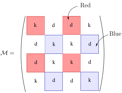
Analyzing the structure of Q one can establish how a generic matrix Mis split into 2×2 blocks each of them giving rise either to kinematical or dynamical gen-erators. This splitting of M is shown in Figure 1, where the kinematical blocks are denoted by k and the dynamical ones by d respectively. Furthermore, one can see that the blocks which are colored in red and blue give rise to charges which are independent of x+ = τ; by this reason these charges commute with the
Hamilto-nian. Complementary, we note that the uncolored both kinematical (fermionic) and dynamical (bosonic) generators do depend on x+.
These conclusions about the structure ofM can be easily drawn by noting that Λ in eq.(3.2) is built out of two commuting matrices Σ+ and Σ− (see (3.3)). For
d
k
k
k d
d
d
d k
k
k
k d
d
k d
M=
Red
[image:10.612.190.426.74.253.2]Blue
Figure 1: The distribution of the kinematical and dynamical charges in theM superma-trix. The red (dark) and blue (light) blocks correspond to the subalgebra J of psu(2,2|4) which leaves the Hamiltonian invariant.
[Σ−,Mkin]=0 and, therefore, due to the structure of QM, see eq.(3.5), the variable
x− cancels out in QM. Explicitly one finds the following conjugation expressions with Λ of (3.2)
Λ−1ModddynΛ =e−i2x−Σ−Modd
dyn, Λ−1Mevendyn Λ = Λ2Mevendyn ,
Λ−1Modd
kin Λ =ei x+Σ+Moddkin , Λ−1Mevenkin Λ =Mevenkin
showing that thex+ =τ independent matrices are indeed given byModddyn andMevenkin ,
i.e. by the red and blue entries in Figure 1.
Finally, we note that the Hamiltonian itself can be obtained from Q as follows
H =−i
2str (QΣ+). (3.6) Another integral of motion, P+, is given by
P+ = i
4str(QΣ−). (3.7)
The structure of Q discussed above is found for finite r and it also remains valid in the limit r → ∞.
3.2 Moment map and the Poisson brackets
are now able to study the Poisson algebra of the Noether charges corresponding to the infinitesimal global symmetry transformations generated by the Lie algebra
psu(2,2|4). Primarily we are interested in those charges which leave the gauge-fixed Hamiltonian and, as the consequence, the symplectic structure of the theory invariant; the corresponding subspace inpsu(2,2|4) will be called J.
Since the symplectic form ω remains invariant under the action of J, to ev-ery element M ∈ J one can associate a locally Hamiltonian phase flow ξM whose Hamiltonian function is nothing else but the Noether charge QM:
ω(ξM, . . .) + dQM= 0. (3.8)
Identifying psu(2,2|4) with its dual space, psu(2,2|4)∗, by using the supertrace
op-eration, we can treat the matrix Q as the moment map [27] which maps the phase space (x, p, χ) into the dual space to the Lie algebra:
Q : (x, p, χ)→psu(2,2|4)∗
and it allows one to associate to any element of psu(2,2|4) a function QM on the phase space. This linear mapping from the Lie algebra into the space of functions on the phase space is given by eq.(3.5). The function QM appears to be a Hamiltonian function, i.e. it obeys eq.(3.8), only if M ∈ J. Although the elements of psu(2,2|4) which do not belong to J are the symmetries of the gauge-fixed action, they leave invariant neither the Hamiltonian nor the symplectic structure.
As is well known [28, 29], eq.(3.8) implies the following general formula for the Poisson bracket of the Noether charges QM
{QM1,QM2} = (−1)
π(M1)π(M2)str(Q[M
1,M2]) + C(M1,M2), (3.9)
where M1,2 ∈ J. Here π is the parity of a supermatrix and [M1,M2] is the graded
commutator, i.e. it is the anti-commutator if both M1 and M2 are odd matrices,
and the commutator if at least one of them is even. The first term in the r.h.s. of eq.(3.9) reflects the fact that the Poisson bracket of the Noether charges QM1 and
QM2 gives a charge corresponding to the commutator [M1,M2]. The normalization
prefactor (−1)π(M1)π(M2) is of no great importance and, as we will see later on, it is
related to our specific choice of normalizing the even elements with respect to the odd ones inside the matrix Q. The quantity C(M1,M2) in the r.h.s. of eq.(3.9) is the
central extension, i.e. a bilinear graded skew-symmetric form on the Lie algebra J which Poisson-commutes with all QM, M ∈ J. The Jacobi identity for the bracket (3.9) implies that C(M1,M2) is a two-dimensional cocycle of the Lie algebraJ. For
Some comments are necessary here. As we already mentioned in section 2, the usual feature of closed string theory considered in the light-cone gauge is the presence of the level-matching constraintpws = 0. This constraint arises from the requirement
of the unphysical field x− to be a periodic function of the world-sheet coordinate
σ. The level-matching constraint cannot be solved in classical theory, rather it is required to vanish on physical states. Thus, before we turn our attention to the question of the physical spectrum we should treat pws as a non-trivial variable. We
will refer to a theory with a non-vanishing generatorpwsas theoff-shelltheory. Since
the Hamiltonian contains only physical fields it commutes with pws: {H, pws} = 0,
i.e. the momentum pws is an integral of motion. The Poisson bracket (3.9) with
the vanishing central term is valid on-shell and it is the off-shell theory where one could expect the appearance of a non-trivial central extension. Below we determine a general form of the central extension based on symmetry arguments only and in the next section by explicit evaluation of the Poisson brackets we justify the formula (3.9) and also find a concrete realization of C(M1,M2).
Let us note that a formula as (3.9) makes it easy to reobtain our results on the structure of J. Indeed, from eq.(3.9) we find that the invariance subalgebra
J ⊂psu(2,2|4) of the Hamiltonian is determined by the condition
{H,QM}= str(Q[Σ+,M]) = 0.
Thus, J is the stabilizer of the element Σ+ inpsu(2,2|4):
[Σ+,M] = 0, M ∈ J .
Obviously, J coincides with the red-blue submatrix ofM in Figure 1. Thus, forP+
being finite5 we would obtain the following vector space decomposition of J
J =psu(2|2)⊕psu(2|2)⊕Σ+⊕Σ−.
The rank of the latter subalgebra is six and it coincides with that of psu(2,2|4). In the case of infinite P+ the last generator decouples.
Now we are ready to determine the general form of the central term in eq.(3.9). Denote by Jeven ⊂ J the even (bosonic) subalgebra of J. It is represented by the
red and blue diagonal blocks in Figure 1. LetGevenbe the corresponding group. The
adjoint action of Geven preserves the Z2-grading of J. Obviously, if we perform the
transformation
Q→gQg−1, M →g−1Mg
5As a side remark, we note that forP
+ finite the subalgebra which leaves invariant both H and
P+ coincides with the even (bosonic) sublagebraJeven ofJ. According to eqs.(3.6) and (3.7), this
subalgebra arises as the simultaneous solution the two equations, [Σ+,M] = 0 and [Σ−,M] = 0,
with an element g ∈ Geven the charge QM remains invariant. This transformation
leaves the l.h.s of the bracket (3.9) invariant. Thus, the central term must satisfy the following invariance condition:
C(gM1g−1, gM2g−1) = C(M1,M2). (3.10)
It is not difficult to find a general expression for a bilinear graded skew-symmetric form on J which satisfies this condition. It is given by
C(M1,M2) = str
̺M1̺Mt2+ (−1)π(M1)π(M2)̺M2̺Mt1
∆
. (3.11)
Here
∆ = −1 2
c3I2 0 0 0
0 c1I2 0 0
0 0 c4I2 0
0 0 0 c2I2
, (3.12)
where I2 is the two-dimensional identity matrix and
̺=
σ 0 0 0 0 σ 0 0 0 0 σ 0 0 0 0 σ
, σ =
0 1
−1 0
. (3.13)
Condition (3.10) follows from the form of the matrix ∆ and the equation
Jevent ̺+̺Jeven = 0. (3.14)
The coefficientsci,i= 1, . . . ,4 can depend on the physical fields and they are central
w.r.t. the action of J:
{ci,QM}= 0, M ∈ J .
By using eq.(3.11) one can check that the cocycle condition for C(M1,M2) is trivially
satisfied. In accordance with our assumptions, C(M1,M2) does not vanish only if
bothM1 and M2 are odd.
Taking into account thatJ contains two identical subalgebras psu(2|2) we can put c1 = c3 and c2 = c4. Thus, general symmetry arguments fix the form of the
central extension up to two central functionsc1 andc2. Since we consider the algebra psu(2,2), which is the real form of psl(2|2), the conjugation rule implies that c1 =
−c∗
2. In the next section we compute the Poisson brackets of the Noether charges
and determine the explicit form of c≡c1.
3.3 Explicit basis
basis elements. Since J contains two identical psu(2,2) sublagebras it is enough to analyze the Poisson brackets corresponding to one of them. For definiteness, we concentrate our attention on the subalgebrapsu(2,2)Rwhich is represented in Figure
1 by blue (right) blocks. For this subalgebra we select a basis in which the fermionic (dynamical) generators are given by
Q11 =
1 2str Qσ
+⊗(Γ
14−Γ23+P−) , Q12 = str Qσ+⊗Γ13,
Q2 2 = −
1 2str Qσ
+⊗(Γ
14−Γ23− P−) , Q12 =−str Qσ+⊗Γ42 (3.15)
and their conjugate charges ¯Qα a are
¯
Q11 =−1 2str Qσ
−⊗(Γ
14−Γ23+P−) , Q¯12 =−str Qσ−⊗Γ13,
¯
Q22 = 1 2str Qσ
−⊗(Γ
14−Γ23− P−) , Q¯21 = str Qσ−⊗Γ42. (3.16)
On the other hand, the bosonic (kinematical) charges are defined as
L1 1 =
i
2str QP
+
2 ⊗(Γ14−Γ23) , L22 =−L11,
L12 =−istr QP2+⊗Γ13, L21 =−istr QP2+⊗Γ24, (3.17)
and
R1 1 =
i
2str QP
−
2 ⊗(Γ14−Γ23) , R22 =−R11,
R12 = istr QP2−⊗Γ13, R21 =istr QP2−⊗Γ24, (3.18)
We refer the reader to the appendix 6.1. for notations used here.
Rewriting the bracket (3.9) in this basis we obtain the following relations
{Ra
b, Jc} = δcbJa−
1 2δ
a
bJc, {Lαβ, Jγ}=δ γ βJα−
1 2δ
α βJγ,
{Qαa,Q¯bβ} = δabLαβ +δβαRab +1 2δ
b aδβαH,
{Qα
a, Qβb} = ǫαβǫab c , {Q¯αa,Q¯bβ}=ǫabǫαβ c∗. (3.19)
Here in the first line we have indicated how the indices a and γ of any Lie algebra generator transform under the action of the bosonic subalgebras generated by Ra b
and Lα
β. In the next section we are going to derive the so far undetermined central
function cin terms of physical variables of string theory.
4. Deriving the central charges
of the classical and quantum supersymmetry algebra does not seem to be feasible. Hence, simplifying perturbative methods need to be applied. The perturbative ex-pansion of the supersymmetry generators in powers of ζ = √2π
λ or, equivalently, in
the number of fields defines a particular expansion scheme. This expansion, however, does not allow one to determine the exact form of the central charges because they are also expected to be non-trivial functions of ζ. To overcome this difficulty in this section we describe a “hybrid” expansion scheme which can be used to determine the exact form of the central charges. To be precise we determine only the part of the central charges which is independent of fermionic fields. We find that this part depends solely on the piece of the level-matching constraint which involves the bosonic fields. Since the central charges must vanish on the level-matching constraint surface, the exact form of the central charges is, therefore, unambiguously fixed by its bosonic part.
More precisely, a dynamical supersymmetry generator has the following generic structure
QM =
Z
dσ eiαx−Ω(x, p, χ;ζ). (4.1)
Depending on the supercharge, the parameter α in the exponent of (4.1) can take two values α = ±1
2. Here the function Ω(x, p, χ;ζ) is a local function of transverse
bosonic fields and fermionic variables. It depends onζ, and can be expanded, quite analogous to the Hamiltonian, in power series
Ω(x, p, χ;ζ) = Ω2(x, p, χ) +ζΩ4(x, p, χ) +· · ·
Here Ω2(x, p, χ) is quadratic in fields, Ω4(x, p, χ) is quartic and so on. Clearly, every
term in this series also admits a finite expansion in number of fermions. In the usual perturbative expansion we would also have to expand the non-local “vertex” eiαx−
in powers ofζ becausex′
− ∼ −ζpx′+· · ·. In the hybrid expansion we do not expand
eiαx− but rather treat it as a rigid object.
a field redefinition which can be determined up to any given order inζ. Taking into account the field redefinition, integrating by parts if necessary, and using the relation
x′
− ∼ −ζpx′+· · ·, one can cast any supercharge (4.1) to the following symbolic form
QM =
Z
dσ eiαx−χ· Υ
1(x, p) +ζΥ3(x, p) +· · ·
+O(χ3), (4.2)
where Υ1 and Υ3 are linear and cubic in bosonic fields, respectively. The explicit
form of the supercharges expanded up to the orderζ can be found in the Appendix.
It is clear now that the bosonic part of the Poisson bracket of two supercharges is of the form
{Q1,Q2} ∼
Z ∞
−∞
dσ ei(α1+α2)x−
Υ(1)1 (x, p)Υ(2)1 (x, p) (4.3)
+ζ Υ(1)1 (x, p)Υ(2)3 (x, p) + Υ3(1)(x, p)Υ(2)1 (x, p)+· · ·,
where Q1,2 ≡ QM1,2. Computing the product Υ (1)
1 (x, p)Υ (2)
1 (x, p) in the case α1 = α2 =±1/2, we find that it is given by
Υ(1)1 (x, p)Υ(2)1 (x, p)∼ 1
ζx
′ −+
d
dσf(x, p), (4.4)
where f(x, p) is a local function of transverse coordinates and momenta. The first term in (4.4) nicely combines withe±ix− to give d
dσe±ix−, and integrating this
expres-sion over σ, we obtain the sought for central charges
Z ∞
−∞
dσ d dσe
±ix− =e±ix−(∞)
−e±ix−(−∞) =e±ix−(−∞) e±ipws−1 , (4.5)
where we take into account that x−(∞)−x−(−∞) =pws.
Making use of the particular basis described in the previous section and imposing the boundary conditionx−(−∞) = 0, we identify the exact expression for the central function cin eqs.(3.19):
c= 1 2ζ(e
ipws −1). (4.6)
The algebra (3.19) with the central charges of the form (4.6) perfectly agrees with the one considered in [5] in the field theory context.
It is worth noting that there is another natural choice of the boundary condition for the light-cone coordinate x−:
This is the symmetric condition which treats both boundaries on the equal footing, and leads to a purely imaginary central charge
c= i
ζ sin( pws
2 ). (4.7)
It is obvious from (4.5) that different boundary conditions for x− lead to central charges which differ from each other by a phase multiplication. This freedom in the choice of the central charge follows from the obvious U(1) automorphism of the algebra (3.19): one can multiply all supercharges Qα
a by any phase which in general
may depend on all the central charges.
Since we already obtained the expected central charges, the contribution of all the other terms in (4.3) should vanish. Indeed, the second term in (4.4) contributes to the order ζ in the expansion as can be easily seen integrating by parts and using the relation x′
− ∼ −ζpx′ +· · ·. Taking into account the additional contribution to
the terms of order ζ in (4.3), we have checked that the total contribution is given by a σ-derivative of a local function of x and p, and, therefore, only contributes to terms of order ζ2.
We have verified up to the quartic order in fields that the Poisson bracket of supercharges with α1 =−α2 gives the Hamiltonian and the kinematic generators in
complete agreement with the centrally extended su(2|2) algebra (3.19).
The next step is to show that the Hamiltonian commutes with all dynamical supercharges. As was already mentioned, this can be done order by order in pertur-bation theory in powers of the inverse string tension ζ and in number of fermionic variables. We have demonstrated that up to the first non-trivial order ζ the super-charge Q truncated to the terms linear in fermions indeed commutes with H. To do that we need to keep in H all quadratic and quartic bosonic terms, and quadratic and quartic terms which are quadratic in fermions, see the Appendix for details.
The computation we described above was purely classical, and one may want to know if quantizing the model could lead to some kind of an anomaly in the symmetry algebra. We have computed the symmetry algebra in the plane-wave limit where one keeps only quadratic terms in all the symmetry generators, and shown that all potentially divergent terms cancel out and no quantum anomaly arises. As a result, one gets again the same centrally extended su(2|2) algebra (3.19) with the central charges 1/ζ(e±ipws−1) replaced by their low-momentum approximations
∓iR−∞∞ dσpMx′M − 2istr(Σ+χχ′)
.
Thus, we have shown that in the infiniteP+ limit and for physical fields chosen
5. Concluding remarks
The main focus of this paper has been on the analysis of the off-shell string sym-metry algebra in the limit of infinite light-cone momentum P+. Relaxing the
level-matching condition brings only one modification in this case: namely, the algebra
psu(2|2)⊕psu(2|2) undergoes extension by a new central charge proportional to the level-matching condition.
The physically more relevant situation, however, corresponds to the case of a finite light-cone momentum. For P+ finite the zero mode of the conjugate field x−
has to be taken into account. Also, since the length of the string is finite, transverse fields do not have to vanish at the string end points. So the question arises what is the symmetry algebra in this case?
Recall that relaxing the level-matching condition for finite P+ means
x−(r)−x−(−r) =pws, −r≤σ ≤r , r= πP+
√
λ ,
which implies that the Poisson bracket of the dynamical supercharge Q, eq.(4.1), with the level-matching generator is
1
ζ{pws,Q}=
Z r
−r
dσ ∂σQ = Ω(r)eiαx−(−r)(eiαpws −1)6= 0.
Hence this Poisson bracket does not vanish, since Ω(r) = Ω(−r) is non-zero in the finite P+ case. Similarly the Poisson bracket of the same supercharge with the
Hamiltonian will be non-vanishing. Thus, we see that the off-shell extension of the theory does not allow one to maintain the psu(2,2|4) symmetry algebra for a string of finite length.
It should be further noted that an off-shell theory is not uniquely defined. Indeed, one can use the level-matching generator to modify the Hamiltonian
H→H +cnpnws,
where the coefficientscnmight depend on physical fields. On the states satisfying the
condition of level-matching the new Hamiltonian reduces to the original one. The absence of the standardpsu(2,2|4) symmetry in an off-shell theory does not a priory preclude the existence of new hidden symmetries of the off-shell Hamiltonian. Their discovery would provide a substantial step in understanding the string dynamics for the physically relevant situation of the finite light-cone momentum.
In the hybrid expansion used in our paper, the crucial role in deriving the non-linear central charges, was played by the “vertex” eiαx−
the physical meaning of this object? To see this, consider the quantum theory. The variable x−(s) contains a zero mode1 xˆ
− which is conjugate to the operator ˆP+
[ ˆP+,xˆ−] =−i .
Thus, if we consider a state |P+i with a definite value of ˆP+|P+i = P+|P+i then a
state eiαˆx−|P
+i carries a new value ofP+:
ˆ
P+eiαx−|P
+i= (α+P+)eiαx−|P
+i
Since in the light-cone approach P+ is naturally identified with the length of the
string, it is appropriate to calleiαx− the length-changing operator. The Hilbert space
of the corresponding theory is necessarily a direct sum: H=PP+HP+ of the spaces
HP+ corresponding to an individual eigenvalue of the operator ˆP+.
This brief discussion of the light-cone string theory for finiteP+ clearly
demon-strates that the latter carries many subtleties with respect to the infinite P+ limit,
which for sure require further investigation.
Acknowledgements
We wish to thank Niklas Beisert for valuable discussions. The work of G. A. was supported in part by the RFBI grant N05-01-00758, by NWO grant 047017015 and by the INTAS contract 03-51-6346. The work of G. A. and S. F. was supported in part by the EU-RTN network Constituents, Fundamental Forces and Symmetries of the Universe (MRTN-CT-2004-005104). The work of J. P. is supported by the Volkswagen Foundation. He also thanks the Albert-Einstein-Institute for hospitality. The work of M. Z. was supported in part by the grantSuperstring Theory (MRTN-CT-2004-512194). M. Z. would like to thank the Spinoza Insitute for the hospitality during the last phase of this project.
6. Appendix
6.1 The gauge-fixed Hamiltonian
The Hamiltonian for physical excitations arising in the light-cone gauge was found in [11]. The gauge choice made in [11] is however not exactly the same as eq.(2.2) adopted here. Also the theory in [11] is defined on the standard interval for σ:
−π ≤ σ ≤ π. In order to make a connection with the results by [11] we choose the variable p+ there to be equal to p+ = 2P+, where P+ is identified with the
total momentum in (2.3). To justify our choice we note that with p+ = 2P+ the
gauge-fixed action of [11] can be schematically represented in the form
S =P+
Z π
−π
dσdτ
2π
pMx˙M +χ†χ˙ − H
, (6.1)
whereHis theP+-independent Hamiltonian density, (xM, pM) with M = 1, . . . ,8 are
transverse coordinates and their conjugate momenta, and χ encodes the fermionic variables. Since we are interested in the limit of infinite P+, it is appropriate to
make a rescaling σ→ √Pλ
+σ. Upon this rescaling the action (6.1) turns precisely into
eq.(2.4) of the present paper with r = √π
λP+. As was discussed in section 2, we
further supplement this rescaling of σ with rescalings of physical variables
(xM, pM, χ)→
p
ζ(xM, pM, χ). (6.2)
This is necessary in order to ensure to have canonical Poisson brackets for physical fields.
Upon these redefinitions the Hamiltonian found in [11] turns into the one given by eq.(2.6) Explicitly, the quadratic piece of the Hamiltonian density in eq.(2.6) has the form
H2 =
1 2p 2 M + 1 2x 2 M + 1 2x ′2 M + 1
2str(Σ+χKχ˜
′tK) + 1
2strχ
2, (6.3)
while the quartic one is [11]
H4 =
1 4
h
p2yz2−p2zy2+ (y′2z2−z′2y2) + 2(z′2z2−y′2y2) + + str(z2−y2)χ′χ′+ 1
2[Σ
′(x),Σ(x)](χχ′ −χ′χ)−2Σ(x)χ′Σ(x)χ′
+ i 4str
[Σ(x),Σ(p)]′( ˜KχtKχ−χKχ˜ tK) i+O(χ4), (6.4)
where by O(χ4) we encode all the terms which are quartic in fermions (stated in
[11]). The transverse bosonic fields we have denoted as xM = (za, ys) with za (a =
1,2,3,4) accounting for the transverse AdS5 andys (s= 1,2,3,4) for theS5 degrees
of freedom. Prime denotes ∂σ and in the fermionic sector we have introduced the
following notation
K =
K4 0
0 K4
, Ke =
K4 0
0 −K4
.
with the matrixK4 satisfying K42 =−I given by
K4 =
0 1 0 0
−1 0 0 0 0 0 0 1 0 0 −1 0
We also use the notation Σ(x) = ΣMxM and Σ(p) = ΣMpM. The 8×8 matrices ΣM
have the following structure
ΣM =
γa 0
0 0
,
0 0 0iγs
(6.5)
and are written in terms of the four Dirac matrices γi. We work with the basis
defined in appendix A of [11]. For the definition of the matrices Σ± see eq.(3.3).
The fermions enter in the above through theκ-gauge fixed 8×8 matrix χ (com-pare (A.6) and (A.9) of [11])
χ=
0 P+η+P−θ†
−P−η†+P+θ 0
, P+=
I2 0
0 0
, P− =
0 0 0 I2
(6.6) where η = 4 X i=1 ˜
ηiΓi, θ = 4
X
i=1
˜
θiΓi, (6.7)
with the Dirac matrices Γi in the complex basis defined in [11], explicitly
Γ1 = 12(γ2−iγ1) =
0 0 0 i
0 0 0 0 0 −i 0 0 0 0 0 0
, Γ2 =
1
2(γ4−iγ3) =
0 0 −i 0 0 0 0 0 0 0 0 0 0 −i 0 0
and Γ4 = (Γ1)†, Γ3 = (Γ2)†. Moreover we define the standard double index Dirac
matrices by Γab := 12[Γa,Γb]. We also define two-dimensional projectors
P2+ =
1 0 0 0
; P2−=
0 0 0 1
. (6.8)
6.2 Symmetry generators
To describe the symmetry generators Q and the gauge-fixed Hamiltonian we have to introduce a proper parametrization of the coset space SO(4,1)PSU(2,2×SO(5)|4) . Following [11] we chose the coset representative in the form
g(χ, x, t, φ) = Λ(t, φ)g(χ)g(x).
Here xM = (za, yi) is a short-hand notation for the transverse bosonic fields and χ
denotes the 16 physical fermions which are left upon fixing the κ-symmetry. The matrix Λ(t, φ) was defined in (3.2). The element g(x) is the 8×8 matrix which has the following structure in terms of 4×4 blocks related to the AdS and to the sphere parts respectively
g(x) =
1
q
1−ζz2
4
1 + √2ζzaγa
0
0 q 1
1+ζy2
4
1 + i√2ζyiγi
Finally the fermionic coset element reads [11]
g(χ) = pζ χ+p1 +ζ χ2.
The 8×8 supermatrix Q of (3.1) is then defined by [11]
Q =
Z r
−r
dσ ΛUΛ−1, (6.9)
where
U =g(χ)g(x)
π
+ i2g(x)KFe
t
σKg(x)−1
g(x)−1g(χ)−1. (6.10)
HereK and ˜K have been defined above. We also have
Fσ =
p
ζ(p1 +ζχ2∂
σχ−χ∂σ
p
1 +ζ χ2)
and
π
is defined byπ
= i4
π
+Σ++i
4
π
−Σ−+ 12
π
MΣM , whereπ
+=1
G+
(2 +G−
π
−),π
−=− G+(π
2
M + A2)
(1 +p1−G+G−(
π
2M + A2)) ,π
a=p
ζ pa(1−ζ z2
4 ),
π
s=p
ζ ps(1 +ζ y2
4). Finally A2 and G
± are given by
A2 =−x′2
−G+G−+
ζz′2 a
1−ζz2 4
2 +O(χ
2), G
±=
1 2
1 +ζz42
1−ζz42 ±
1−ζy42
1 +ζy42
!
.
6.3 Covariant notation
As was done in [11] we shall make use of complex fields. However, here we will denote them in a covariant notation with upper and lower indices reflecting their charges under the four transverse U(1) subgroups involved. The bosonic fields we denote by
Z1 =z2 +iz1; Z2 =z4+iz3; Z2 = (Z2)†; Z1 = (Z1)†; Y1 =y2+iy1; Y2 =y4+iy3; Y2 = (Y2)†; Y1 = (Y1)†;
P1Z = 12(pz2+ip1z) ; P2Z = 12(pz4+ipz3) ; (PZ)1 = (P1z)†; (PZ)2 = (P2Z)†;
P1Y = 1 2(p
y 2+ip
y
1) ; P2Y = 12(p y 4 +ip
y
3) ; (PY)1 = (P1Y)†; (PY)2 = (P2Y)†.
with the quantum commutation relations (α, β = 1,2 anda, b= 1,2)
[PαZ(σ), Zβ(σ′)] =−i δαβδ(σ−σ′) [(PZ)α(σ), Zβ(σ′)] =−i δβαδ(σ−σ′)
[PaY(σ), Yb(σ′)] =−i δabδ(σ−σ′) [(PY)a(σ), Yb(σ′)] =−i δbaδ(σ−σ′),
analogue expressions apply at the classical level for the Poisson brackets.
We also introduce upper and lower indices for the fermionic fields defined in (6.7) by denoting
˜
θ1 =θ1 θ˜2 =θ2 θ˜3 =θ2 θ˜4 =θ1
˜
θ1†=θ†1 θ˜†2 =θ†2 θ˜3†=θ†2 θ˜4†=θ1†
˜
η1 =η1 η˜2 =η2 η˜3 =η2 η˜4 =η1
˜
η1†=η†1 η˜†2 =η†2 η˜3†=η2† η˜4†=η†1,
(6.12)
leading to the covariant anti-commutation relations
{θα(σ), θ†β(σ′)}=δαβδ(σ−σ′) {θα(σ), θ†β(σ′)}=δβαδ(σ−σ′)
{ηa(σ), η†b(σ′)}=δabδ(σ−σ′) {ηa(σ), η†b(σ′)}=δbaδ(σ−σ′).
(6.13)
It is useful to note the charges carried by the fields of the four U(1) subgroups involved. For this consider the combinations S± =S1±S2 and J± =J1±J2. Then
the su(2|2)R right (blue) generators carry J− and S− charges whereas the su(2|2)L
left (red) generators are charged under S− and J−. The following tables exemplify this:
S+ S− J+ J−
Z1, (PZ)1, Z¯1,( ¯PZ)1, 1 1 0 0 Z2, (PZ)2, Z¯2, ( ¯PZ)2, 1 −1 0 0 Z2, (PZ)2, Z¯
2, ( ¯PZ)2, −1 1 0 0 Z1, (PZ)1, Z¯1, ( ¯PZ)1, −1 −1 0 0 ,
S+ S− J+ J−
Y1, (PY)1, Y¯1, ( ¯PY)1, 0 0 1 1 Y2, (PY)2, Y¯2, ( ¯PY)2, 0 0 1 −1 Y2, (PY)2, Y¯
2, ( ¯PY)2, 0 0 −1 1 Y1, (PY)1, Y¯1, ( ¯PY)1, 0 0 −1 −1
S+ S− J+ J−
θ1, θ1†, θ¯1, θ¯1†, 0 1 1 0 θ2, θ†2, θ¯2, θ¯†2, 0−1 1 0 θ2, θ†2,θ¯
2,θ¯†2, 0 1 −1 0 θ1, θ†1, θ¯1, θ¯†1, 0−1 −1 0
,
S+ S− J+ J−
η1, η1†,η¯1, η¯†1, 1 0 0 1 η2, η2†, η¯2, η¯†2, 1 0 0 −1 η2, η†2, η¯
2, η¯2†, −1 0 0 1 η1, η†1,η¯1, η¯†1, −1 0 0 −1
Hence a lower (upper) index on Z, Y, PZ, PY, θ, η, θ† and η† denotes a charge of 1
(-1) with respect to (S++J+). In the above tables we have also introduced barred
coordinates defined with a flipped “2” index as
¯
A1 =A1, A¯1 =A1, A¯2 =A2, A¯2 =A2, with A∈ {Z, Y, PZ, PY, θ, η, θ†, η†},
which are the natural objects for the su(2|2)L left (red) generators as we shall see
6.4 The explicit form of the su(2|2)R generators
Using the basis of fermionic (dynamical) generators of the right (blue)su(2|2)R
alge-bra given in (3.15) and (3.16) along with the concrete expression for Q in (6.9) one finds the leading quadratic order expressions for the supercharges
Qαa=−
1 2
Z
dσ e−i2x−
h
i θα(2PY +iY)a+ (2PZ−iZ)αηa†−θ†αYa′−iZ′αηa
+ǫαβǫab
iθβ(2PY +iY)b+ (2PZ−iZ)βη†b−θ†βY′b−i Zβ′ ηb
i
(6.14)
¯
Qαa =
1 2
Z
dσ ei2x−
h
iθ†α(2PY −iY)a−(2PZ+iZ)αηa+θαY′a−iZα′ η†a
+ǫαβǫab
iθ†β(2PY −iY)
b−(2PZ+iZ)βηb+θβYb′−i Z′βη†b
i
= (Qα a)†.
(6.15)
Moreover thesu(2) generatorsRα
β andLab can be computed using the basis of (3.17)
and (3.18). They read
Rαβ =
Z
dσi[(PZ)αZβ −(PZ)βZα] + i
2δ
α
β[(PZ)γZγ−(PZ)γZγ]
+θ†βθα−θ†αθβ +
1 2δ
α
β [θ†γθγ−θ†γθγ]
(6.16)
Lab =
Z
dσi[(PY)aYb−(PY)bYa] + i
2δ
a
b [(PY)cYc −(PY)cYc]
+ηb†ηa−η†aηb+
1 2δ
a
b [η†cηc−ηc†ηc]
. (6.17)
Using the above expressions for the supersymmetry generators, it is straightforward to compute their quantum anti-commutators. One indeed finds
{Qαa,Q¯βb}=δabRαβ+δβαLba+
1 2δ
b
aδβαH (6.18)
with the Hamiltonian
H = 2
Z
dσh(PZ)γ(PZ)γ+ (PY)c(PY)c +
1 4(Z
γZ
γ+Z′γZγ′ +YcYc+Y′cYc′)
+ 1 2(θ
†γθ
γ+θ†γθγ+η†cηc+ηc†ηc) +
1 2(θ
†′
γθ†γ−θ′γθγ+ηc†′η†c−η′cηc)−2δ(0)
i
.
(6.19)
The normal ordering contribution −2δ(0) of the fermions will cancel against the ground state energy of the bosons by supersymmetry upon introduction of creation and annihilation operators.
The su(2) generators Rα
β and Lab (6.17) and (6.16) can be shown to obey the
commutation relations
Next we turn to the quantum anticommutator {Qα
a, Qβb} which evaluates to
{Qαa, Qβb}= i
2ζ ǫ αβǫ
ab
Z
dσ e−i x−x′ −+
Z
dσ1dσ2δ(σ1−σ2) (∂σ1 +∂σ2)δ(σ1 −σ2)
We see that the potential last quantum anomaly cancels and we recover the central charge announced in (3.19) also at the quantum level. The analogous computation for {Q¯α
a,Q¯βb}follows from conjugation.
Finally let us stress that in the above computations we have freely performed partial integrations by dropping contributions arising from the vertex operatorse±ix−,
as these would take us beyond the leading quadratic field approximation. These terms where dealt with, however, at the classical level up to orderO(ζ) as discussed in section four.
6.5 The su(2|2)R supercharge at quartic field order
Here we spell out the contribution to the right (blue) supercharges at quartic field order (O(ζ2)) explicitly, restricting to the terms linear in fermions whose Poisson
brackets yield the quartic bosonic Hamiltonian
Qaα
f bbb=
Z
dσe−i x−/2
n
(θαYa+ǫαβǫabθβYb) [−4i (PY)◦Y − 12Hbos]
+θα(2PY −iY)a+ǫαβǫabθβ(2PY −iY)b
[i
4 Y ◦Y]
+ (θ†αYa+ǫαβǫabθβ†Yb) [4i (P
Y ◦Y′+PZ◦Z′) + 1
4Z◦Z′− 1
8Y ◦Y′]
+ (θ†αYa′+ǫαβǫabθ†βY′b) [12Z◦Z− 1
4Y ◦Y]
+ (ηa†Zα+ǫαβǫabη†bZβ) [−14(PZ)◦Z +2i Hbos]
+ηa†(2PZ+iZ)α+ǫαβǫabη†b(2PZ+iZ)β
[14Z◦Z]
+ (ηaZα+ǫαβǫabηbZβ) [14(PY ◦Y′+PZ◦Z′)−4i Y ◦Y′+8i Z ◦Z′]
+ (ηaZ′α+ǫαβǫabηbZβ′ ) [−2i Y ◦Y + i
4Z ◦Z]
o
, (6.21)
where we have used the notation (PZ)◦Z := (PZ)
γZγ+ (PZ)γZγ and (PY)◦Y :=
(PY)
cYc+ (PY)cYc, etc. Also Hbos denotes the bosonic part of the free (quadratic)
Hamiltonian (6.19). Similar expression follow for the left (red) supercharges.
6.6 The explicit form of the su(2|2)L generators
We denote all the generators appearing in the left (red) su(2|2)L algebra by lower
supercharges we take as a basis
q11 =
1
2str Qσ
+⊗(Γ
14+ Γ23+P+)
q22 =−
1
2str Qσ
+⊗(Γ
14+ Γ23− P+) q12 = str Qσ+⊗Γ12
q21 = str Qσ+⊗Γ34. (6.22)
One then finds at quadratic field order
q11=
1 2
Z
dσ eix−/2
h
(2PZ+iZ)γθγ+i Z′γθ†γ+i(2PY −iY)cη†c+Yc′ηc i
q22=
1 2
Z
dσ eix−/2
h
(2PZ+iZ)γθγ+i Zγ′ θ†γ+i(2PY −iY)cηc†+Y′cηc i
q12= 1
2
Z
dσ eix−/2
h
ǫαβ(2PZ+iZ)αθβ+i Z′αθ†β−ǫabi(2PY −iY)aη†b+Y′aηb i
q21=−1
2
Z
dσ eix−/2
h
ǫαβ(2PZ+iZ)αθβ+i Zα′ θ † β
−ǫabi(2PY −iY)aηb†+Ya′ηb i
(6.23)
and their complex conjugated partners ¯qAB. These generators can be shown to
anti-commute with the right (blue) supercharges Qα
a and ¯Qαa, their commutation with
the right (blue)su(2) generatorsRα
β andLab is manifest due to the (right) covariant
notation.
Translating these charges into the barred coordinates with the flipped “2” index of (6.14) enables one to write the left (red) supercharges covariantly
qA B =
1 2
Z
dσ eix−/2
h
(2¯pZ+iZ¯)Aθ¯
B+iZ¯′Aθ¯B† +i(2¯pY −iY¯)Bη¯†A+ ¯YB′ η¯A
+ǫACǫBD
(2¯pZ+iZ¯)Cθ¯D +iZ¯C′ θ¯†D+i(2¯pY −iZ¯)Dη¯C† + ¯Y′Dη¯C
i
(6.24)
and the complex conjugate expression ¯qAB. Here we note the conjugation
proper-ties ( ¯ZA)† = ¯ZA, (¯θA)† = ¯θ†A, (¯pZA)† = (¯pZ)A, etc. One then computes the
anti-commutator
{qAB,q¯CD}=−δCAlDB −δBDrCA+
1 2δ
A
CδDBH (6.25)
bosonic su(2) generators appearing on the right hand side are given by
rAB =i
h
(¯pZ)AZ¯B−(¯pZ)BZ¯A
i + i 2δ A B h
(¯pZ)CZ¯C −(¯pZ)CZ¯C
i
−h(¯η†)Aη¯B−(¯η†)Bη¯A
i +1 2δ A B h
(¯η†)Cη¯C−(¯η†)Cη¯C
i
, (6.26)
lAB =i
h
(¯pY)AY¯B−(¯pY)BY¯A
i + i 2δ A B h
(¯pY)CY¯C −(¯pY)CY¯C
i
−h(¯θ†)Aθ¯B−(¯θ†)Bθ¯A
i +1 2δ A B h
(¯θ†)Cθ¯C −(¯θ†)Cθ¯C
i
. (6.27)
They are traceless and obey thesu(2) algebra.
Finally one again computes the anti-commutator
{qAB, qCD}=− i
2ǫ
ACǫ BD
Z
dσei x−
h
(PZ)◦Z′+ (PY)◦Y′+i(θ†◦θ′+η†◦η′)i
giving rise to the level-matching condition as we had in the right (blue) algebra. We note that the right-hand side of the above takes the same form in barred or unbarred variables.
6.7 The centrality of the level-matching and Hamiltonian
In this section, we show that the level-matching generatorpws and the Hamiltonian
do Possion-commute with all the generators of the su(2|2)⊕su(2|2) algebra. The explicit computation follows the logic of section 4.
Since we would like to work in the limit of infinite P+ we also have to suppress
the corresponding conjugate zero modex−. We pick up a solution for the unphysical field x−(s) which obeys the boundary condition x−(−∞) = 0. It reads as
x−(s) =−ζ
Z s
−∞
dω pMx′M − i
2str(Σ+χχ
′).
Using the canonical Poisson brackets it is easy to find
1
ζ{pM(σ), x−(s)}=δ(σ−s)pM(σ)−p
′
M(σ)ǫ(s−σ),
1
ζ{xM(σ), x−(s)}=−x
′
M(σ)ǫ(s−σ),
1
ζ{x
′
M(σ), x−(s)}=−x′′M(σ)ǫ(s−σ) +x′M(σ)δ(σ−s),
1
ζ{χ(σ), x−(s)}=
1
2δ(σ−s)χ(σ)−χ
′(σ)ǫ(s−σ).
(6.28)
ǫ(s) =
1, s≥0,
0, s <0 , (6.29)
which satisfies the condition ǫ(s) +ǫ(−s) = 1. The reader can easily verify the validity of these formulae by considering, e.g., the Jacobi identity.
First, using these formulae one can check that the supercharges commute with the level-matching generator. Introducing the level-matching generator
pws =−ζ
Z ∞
−∞
dω pMx′M − i
2str(Σ+χχ
′)
it is easy to see that
1
ζ{pws, xM(s)}=x
′
M(s),
1
ζ{pws, pM(s)}=p
′
M(s),
1
ζ{pws, χ(s)}=χ
′(s)
and, therefore,
1
ζ{pws, x−(s)}=−ζ pMx
′
M − i
2str(Σ+χχ
′)(s) = x′ −(s).
Thus,
1
ζ{pws,Q}=
Z
∂sQ = 0
provided all the fields rapidly decrease at infinity.
Note thatx−(s) is quadratic in fermions, while we are interested in the contribu-tion to the Poisson bracket of H and Q which is linear in fermions. This observacontribu-tion implies that computing the Poisson bracket of the Hamiltonian with eiαx−(s) it is
enough to use instead of the full H the quadratic bosonic Hamiltonian with the density Hb
2(σ). Using the basic Poisson brackets it is easy to find
1
ζ{H b
2(σ), x−(s)} = (p2M +x′M2)δ(σ−s)−∂σHb2 ǫ(s−σ).
Finally, to verify the centrality of the Hamiltonian up to orderζ we have to compute
{H,Q} =
Z Z
dσdsh{H2b, eiαx−} Ω
2+
+eiαx− {H
2,Ω2}+ζ{H4,Ω2}+ζ{H2,Ω4}
i
+· · ·
Here the integrals are taken from−∞to +∞and to simplify the notation we do not exhibit the dependence of functions Ω on physical fields. We have
{H,Q} =iαζ
Z
ds eiαx− p2
M +x′M2 − H2b
Ω2
+
Z Z
dσds eiαx− {H
2,Ω2}+ζ{H4,Ω2}+ζ{H2,Ω4}
The further computation is straightforward and it uses explicit expressions for Ω2,4
in terms of transverse fields. We note that the Poisson bracket
{H2,Ω2}+ζ{H4,Ω2}+ζ{H2,Ω4} (6.30)
contains terms proportional to δ(σ−s), δ′(σ−s) and δ′′(σ−s) which reduces the
double integration to a single one. Moreover, according to our assumptions about the orders of perturbation theory we are working on, in the expression (6.30) only the terms linear in fermions should be taken into account. This means, in particular, that in this specific computation only the terms in H4 which are quadratic in fermions
matter. Evaluating the brackets under these assumptions we find that up to the order ζ the integrand appears to be a total derivative and therefore vanishes for fields with rapidly decreasing boundary conditions. Thus, with our assumptions we have verified that
{H,Q}= 0,
i.e. the Hamiltonian commutes with all dynamical supercharges. It is not difficult to extend this treatment to higher orders in fermions and inζ but it is already clear that we will not find any anomaly because of a rigid structure of the supersymmetry algebra: the complete Hamiltonian will commute with all dynamical supercharges.
References
[1] R. R. Metsaev and A. A. Tseytlin, “Type IIB superstring action in AdS5×S5 background,” Nucl. Phys. B533 (1998) 109, hep-th/9805028.
[2] I. Bena, J. Polchinski and R. Roiban, “Hidden symmetries of the AdS5×S5 superstring,” Phys. Rev. D 69(2004) 046002, hep-th/0305116.
[3] G. Arutyunov, S. Frolov and M. Staudacher, “Bethe ansatz for quantum strings,” JHEP 0410, 016 (2004), hep-th/0406256.
[4] M. Staudacher, “The factorized S-matrix of CFT/AdS,” JHEP 0505 (2005) 054, hep-th/0412188. • N. Beisert and M. Staudacher, “Long-range PSU(2,2|4) Bethe ansaetze for gauge theory and strings,” hep-th/0504190.
[5] N. Beisert, “Thesu(2|2) dynamic S-matrix,” hep-th/0511082.
[6] C. G. Callan, H. K. Lee, T. McLoughlin, J. H. Schwarz, I. Swanson and X. Wu, “Quantizing string theory in AdS5×S5: Beyond the pp-wave,” Nucl. Phys. B 673 (2003) 3, hep-th/0307032. • C. G. Callan, T. McLoughlin and I. Swanson,
“Holography beyond the Penrose limit,” Nucl. Phys. B 694 (2004) 115, hep-th/0404007.
692 (2004) 3, hep-th/0403120. •M. Kruczenski and A. A. Tseytlin, “Semiclassical relativistic strings in S5 and long coherent operators in N = 4 SYM theory,” JHEP
0409, 038 (2004), hep-th/0406189.
[8] G. Arutyunov and S. Frolov, “Integrable Hamiltonian for classical strings on AdS5×S5,” JHEP 0502 (2005) 059, hep-th/0411089.
[9] L. F. Alday, G. Arutyunov and S. Frolov, “New integrable system of 2dim fermions from strings on AdS5×S5,” JHEP 0601 (2006) 078, hep-th/0508140.
[10] G. Arutyunov and S. Frolov, “Uniform light-cone gauge for strings in AdS5×S5: Solving su(1|1) sector,” JHEP0601 (2006) 055, hep-th/0510208.
[11] S. Frolov, J. Plefka and M. Zamaklar, “The AdS5×S5 superstring in light-cone gauge and its Bethe equations,” hep-th/0603008.
[12] R. A. Janik, “The AdS5×S5 superstring worldsheet S-matrix and crossing symmetry,” Phys. Rev. D 73(2006) 086006, hep-th/0603038.
[13] G. Arutyunov and S. Frolov, “On AdS5×S5 string S-matrix,” Phys. Lett. B639 (2006) 378, hep-th/0604043. • C. Gomez and R. Hernandez, “The magnon
kinematics of the AdS/CFT correspondence,” hep-th/0608029. •J. Plefka, F. Spill and A. Torrielli, “On the Hopf algebra structure of the AdS/CFT S-matrix,” hep-th/0608038. • N. Beisert, R. Hernandez and E. Lopez, “A crossing-symmetric phase for AdS5×S5 strings,” hep-th/0609044.
[14] N. Mann and J. Polchinski, “Bethe ansatz for a quantum supercoset sigma model,” Phys. Rev. D 72(2005) 086002, hep-th/0508232.
[15] J. Ambjorn, R. A. Janik and C. Kristjansen, “Wrapping interactions and a new source of corrections to the spin-chain / string duality,” Nucl. Phys. B 736 (2006) 288, hep-th/0510171.
[16] G. Arutyunov and A. A. Tseytlin, “On highest-energy state in thesu(1|1) sector of N = 4 super Yang-Mills theory,” JHEP 0605 (2006) 033, hep-th/0603113.
[17] T. Klose and K. Zarembo, “Bethe ansatz in stringy sigma models,” hep-th/0603039.
[18] N. Gromov, V. Kazakov, K. Sakai and P. Vieira, “Strings as multi-particle states of quantum sigma-models,” hep-th/0603043. • N. Gromov and V. Kazakov,
“Asymptotic Bethe ansatz from string sigma model on S3×R,” hep-th/0605026.
[19] D. M. Hofman and J. M. Maldacena, “Giant magnons,” hep-th/0604135.
[20] G. Arutyunov, S. Frolov and M. Zamaklar, “Finite-size effects from giant magnons,” hep-th/0606126.
[21] R. Roiban and W. Siegel, “Superstrings on AdS5×S5 supertwistor space,” JHEP
[22] A. Das, J. Maharana, A. Melikyan and M. Sato, “The algebra of transition matrices for the AdS5×S5 superstring,” JHEP0412 (2004) 055, hep-th/0411200.
A. Das, A. Melikyan and M. Sato, “The algebra of flat currents for the string on AdS5×S5 in the light-cone gauge,” hep-th/0508183.
[23] P. Goddard, J. Goldstone, C. Rebbi and C. B. Thorn, “Quantum dynamics of a massless relativistic string,” Nucl. Phys. B 56(1973) 109.
[24] R. R. Metsaev, C. B. Thorn and A. A. Tseytlin, “Light-cone superstring in AdS space-time,” Nucl. Phys. B 596 (2001) 151, hep-th/0009171.
[25] L.D. Faddeev and L.A. Takhtajan,Hamiltonian methods in the theory of solitons, Springer, 1987.
[26] L. F. Alday, G. Arutyunov and A. A. Tseytlin, “On integrability of classical superstrings in AdS5×S5,” JHEP0507 (2005) 002, hep-th/0502240.
[27] J.M. Souriau,Structure des syst`emes dynamiques, Dunod, 1970.
[28] A.A. Kirillov, Elements of representation theory, in russian, Nauka, 1978.