http://dx.doi.org/10.4236/ajcm.2016.63029
Adaptive Finite Element Method for Steady
Convection-Diffusion Equation
Gelaw Temesgen Mekuria1, Jakkula Anand Rao2
1Department of Mathematics, Mizan Tepi University, Mizan Teferi, Ethiopia 2Department of Mathematics, Osmania University, Hyderabad, India
Received 24 June 2016; accepted 27 September 2016; published 30 September 2016
Copyright © 2016 by authors and Scientific Research Publishing Inc.
This work is licensed under the Creative Commons Attribution International License (CC BY).
http://creativecommons.org/licenses/by/4.0/
Abstract
This paper examines the numerical solution of the convection-diffusion equation in 2-D. The solu-tion of this equasolu-tion possesses singularities in the form of boundary or interior layers due to non-smooth boundary conditions. To overcome such singularities arising from these critical re-gions, the adaptive finite element method is employed. This scheme is based on the streamline diffusion method combined with Neumann-type posteriori estimator. The effectiveness of this ap-proach is illustrated by different examples with several numerical experiments.
Keywords
Convection-Diffusion Problem, Streamline Diffusion Finite Element Method, Boundary and Interior Layers, A Posteriori Error Estimators, Adaptive Mesh Refinement
1. Introduction
in regions where there are layers. One common technique to increase the accuracy of the finite element solution in these critical regions is through local grid refinement, the so-called h-method. The question is how to identify those regions and how to obtain a good balance between the refined and unrefined regions such that the overall accuracy is optimal.
Another related problem is to obtain reliable estimates of the accuracy of the computed numerical solution. A priori estimate are often insufficient and can’t be used to estimate the exact error. Therefore, it is natural to ac-quire a posteriori error estimators to pinpoint where the error is large and, at the same time, properly bound the exact error on the whole domain. The error estimator should be local and should yield reliable upper and lower bounds for the true error in a user-specified norm. Global upper bounds are sufficient to obtain a numerical solu-tion with accuracy below a prescribed tolerance. Local lower bounds are necessary to ensure that the grid is cor-rectly refined so that one obtains a numerical solution with a prescribed tolerance using a nearly minimal num-ber of grid-points.
For two-dimensional problems, several estimators have been shown to be asymptotically exact when used on uniform meshes provided the solution of the problem is smooth enough [6]-[8]. Estimators based on computing residuals, so-called residual-type estimators, and estimators based on solving a local Dirichlet problem, so-called Dirichlet-type estimators, were introduced in [9]. Estimators based on solving a local Neumann problem, so- called Neumann-type estimators, were first given in [10]. These estimators have been studied by many research-ers in [11]-[16]. The Zienkiewicz-Zhu (ZZ) type of estimators based on recovery of gradient and Hessian are also well developed, see [17] & [18], and articles cited therein.
In this paper we introduce and analyze from theoretical and experimental points of view an adaptive scheme to efficiently solve the convection-diffusion equation. This scheme is based on the streamline-diffusion finite element method (SDFEM) introduced in [3] combined with an error estimator similar to the one developed in [14]. We prove global upper and local lower error estimates in the energy norm, with constants which only de-pend on the shape-regularity of the mesh and the polynomial degree of the finite element approximating space. We perform several numerical experiments to show the effectiveness of our approach to capture boundary and inner layers sharply and without significant oscillations.
The paper is organized as follows. In Section 2 we recall the convection-diffusion problem under considera-tion and the Streamline Diffusion Finite Element Method. In Secconsidera-tion 3 we define a posteriori error estimator with the energy norm of the finite element approximation error. Finally, in Section 4, we introduce the adaptive scheme and report the results of the numerical tests.
2. Linear Convection-Diffusion Equation
We consider the following steady linear convection-diffusion equation
2
in
u b u f
− ∇ + ⋅ ∇ = Ω, (2.1a)
on D
u=g Γ , and (2.1b)
0 on N
u n
∂ = Γ
∂ (2.1c) where Ω ⊂2 is a bounded polygonal domain with Lipschitz boundary ∂Ω = ΓDΓN and ΓDΓ = ∅N . We are interested in the convection dominated case and assume that
(A.1) 0≤1, (A.2) ∇ ⋅ =b 0, (A.3) b∞ Ω, =1, (A.4) b n⋅ ≥0. The L2 norm and the
1
H semi-norm (also called Energy Norm) are defined as
( ) ( )
0
2
1 2 2
d
H L
u Ω u Ω u
Ω
= = Ω
∫
and (2.2)( ) ( )
( )
1
2
1 2 2
d
H L
u Ω u Ω u
Ω
= ∇ = ∇ Ω
( )
1
u H
∀ ∈ Ω , respectively. We shall denote the above norm and semi-norm by the following convention
( )
,
.kΩ= u HkΩ and ∇.k,Ω= uk,Ω = uHk( )Ω if no subscript index is given then we assume an ordinary L2
norm, .0,Ω, and if no subscript index is given then we shall assume it is the whole of Ω.
To define weak form of Equation (2.1), we need two classes of functions: the trial functions H1E and the test solutions 10
E H :
( )
{
}
1 1 : D EH = u∈H Ω u=g Γ (2.4)
( )
{
}
0
1 1 : 0
E
H = u∈H Ω u= ∂Ω (2.5) The standard variational formulation of Equation (2.1) is given by: Find u∈H1E such that
( )
,( )
, 10E
B u v =F v ∀ ∈v H (2.6) where
( ) (
, ,) (
,)
B u v = ∇ ∇ + ⋅ ∇ u v b u v and (2.7)
( ) (
,)
F v = f v (2.8)
Let ℑ =h
{ }
K be a decomposition of Ω into triangles.We need to make the following geometrical assumptions on the family of triangulations ℑh
1) Admissibility: whenever K1 and K2 belongs to ℑh, K1K2 is either empty, or reduced to a common
vertex, or to a common edge
1) hk = the diameter of K = the longest side of K∈ ℑh
3) ρk = the supremum of the diameter of the balls inscribed in K∈ ℑh 4) Shape regularity: the ratio of hk to ρk is uniformly bounded i.e.,
, k k h k h K β
ρ ≤ ∀ ∈ ℑ (2.9)
which means for any h>0 and for any K∈ ℑh there exists a constant β >0 0 such that βk ≥β0 where
k
β denotes the smallest angle in any K∈ ℑh. We define the finite element spaces
( )
( )
{
1 1}
: ,
h K h
V = v∈H Ω v ∈P K ∀ ∈ ℑK (2.10) for triangular elements, where 1
( )
P K is the space of polynomials of degree not greater than 1 on K.
In the case of convection-dominated problem, the standard Galerkin approximation of Equation (2.6) may produce unphysical behavior, oscillation, if the mesh is too coarse in critical regions. To circumvent these diffi-culties, stability of the discretization has to be increased by introducing artificial diffusion along streamlines. The Streamline-Diffusion Finite Element Method (SDFEM) [1]-[3] stabilizes a convection-dominated problem by adding weighted residuals to the standard Galerkin finite element method for hyperbolic equations which combines good stability with high order accuracy, convergence results are available (see [19]).
The SDFEM yields the following discrete problem obtained: Find uh∈Vh such that
(
,)
( )
, , 0 onSD h h SD h h h h D
B u v =F v ∀ ∈v V v = Γ (2.11)
where
(
,) (
,) (
,)
(
,)
h
SD h h h h h h K h h K
K
B u v u v b u v δ b u b v
∈ℑ
= ∇ ∇ + ⋅∇ +
∑
⋅∇ ⋅∇ and (2.12)(
,)
(
,)
h
SD h K h K
K
F f v δ f b v
∈ℑ
= +
∑
⋅∇ (2.13)In Equation (2.11), a constant δK must be chosen for every element K. Let the mesh Peclet number be de-
fined by, k ,K k
b h
Pe = ∞
where .∞,K denotes the norm in
(
( )
)
2following choice of δK are optimal; see [20]:
1
1 for 0,
2
0 for 0
k k K k k h Pe Pe Pe δ − > = ≤ (2.14)
where hk is a measure of the element length in the direction of the convection flow b. For other parameter choice, see [21]-[24].
3. A Posteriori Error Estimator
In this topic, we introduce the analysis of a Neumann-type error estimator proposed in [14] which is an exten-sion of the work [25]. In their work, they modify the well-known Bank and Weiser estimator [10] and using the idea of Ainsworth & Oden in [26], they solve a local (element) Poisson problem over a suitably chosen (higher order) approximation space with data from interior residuals and flux jumps along element edges.
We now introduce some definitions and notations that will be needed for the error estimates. We denote by
( )
K the set of edges of element K∈ ℑh, by( )
h h K K ∈ℑ =
the set of all element edges
and the subsets relating to internal, Dirichlet and Neumann edges respectively as
{
}
, :
hΩ = E∈ h E⊂ Ω
, h D, =
{
E∈h:E⊂ ΓD}
and{
}
, :
h N = E∈ h E⊂ ΓN
so that h=h,Ωh D, h N, . We denote K the set of vertices of K∈ ℑh and by
h
h K
K∈ℑ
=
the set of all element vertices (that
do not lie on the Dirichlet boundary ΓD). Let E be the set of vertices of E∈h, and for K∈ ℑh, E∈h and X∈h we define the local “patches” of elements as
( ) ( ) K K K K ′ ≠∅ ′ =
ω , ( ) E E K K ′ ∈ ′ =
ω , K K K K ′≠∅ ′ =
ω , E K E K ′≠∅ ′ =
ωFor the lowest order P1 approximations over a triangular element subdivision, ∇2u K =0, so that the inte-rior residual of element K is given by
(
)
K h K
R = f − ⋅ ∇b u (3.1)
and the internal residual is approximated by
( )
0 0
K K K
R = R (3.2)
where K0 is the L2
( )
K -projection onto( )
0P K .
For any edge E of an element K∈ ℑh, we define the flux jump as
, , , if 2 if 0 if h h E E h
E h N
E h D u E n u R E n E Ω ∂ ∈ ∂ ∂ = − ∈ ∂ ∈ (3.3)
where h E
u n
∂
∂ is a constant function on the inter-element edge E and
[ ]
vE measures the jump of vacross E, that is, for E∈
( )
K ( )
S , K S, ∈ ℑhand defining nE K, and nE S, to be the outward normals with respect to the edge E from element K and S respectively, we haveK =QK ⊕BK
Q (3.5)
consisting of edge and interior bubble functions respectively:
( )
(
)
{
: 0 1, , ,}
K =span ΨE K→ ≤ Ψ ≤E E∈ K hΩ h N
Q (3.6)
where each member of the space is a quadratic (or biquadratic) edge bubble function ΨE that is nonzero on edge E of element K, but non zero valued on all other edges of K.
K
B is the space spanned by interior cubic (or biquadratic) bubbles φK i.e.,
{
: 0 1 , 0 on}
K K K K
B = φ K→ ≤φ ≤ φ = ∂K (3.7) where each function is associated with an element K, and is zero on all edges of K, nonzero on the interior of K, and φ =K 1 at the centeroid of K.
The upshot is that the local problems are always well posed and that for each triangular element a 4 × 4 sys-tem of equations must be solved to compute eK.
For an element K∈ ℑh, the local error estimate is the energy norm of eK given by
K eK K
η = ∇ (3.8)
where eK =
(
u−uh)
K∈QK satisfies(
)
(
)
( )
0 1
, , ,
2
, K K K E E
K K
K E
R v R v
e v v
∈
∇ ∇ = −
∑
∀ ∈
Q (3.9)
In the following, we use the short-hand notation f S to denote L2-norm of a function L2
( )
S . The Kayand Silvester’s a posteriori error estimation can be read as following:
Theorem 1. If the variational Equation (2.6) solved with a grid of linear triangular elements, and if the trian-gle aspect ratio condition is satisfied with βΩ, then, the estimator ηK computed via Equation (3.9) satisfies the (global) upper bound property
( )
1 2 2 2 2 0 h h Kh K K K K
K K
h
e Ω C βΩ η R R
∈ℑ ∈ℑ
∇ ≤ + −
∑
∑
(3.10)where C is independent of and h and hK is the length of the longest edge of element K. Proof. See the details in [14].
Theorem 2. If the variational Equation (2.6) with b∞ =1 is solved via either the Galerkin formulation or the SD formulation Equation (2.11), using a grid of linear triangular elements, and if the triangle aspect ratio condition is satisfied, then the estimator ηK computed via Equation (3.9) is a local lower bound for
(
)
h h
e = u−u in the sense that
( )
0K K
K K
K K
K h h K K K K
K K
h h
c e b e R R
η β
⊂ ⊂
≤ ∇ + ⋅ ∇ + −
ω
∑
∑
ω
ω ω
(3.11)
where c is independent of , and ωK represents the patch of four elements that have at least one boundary edge E from the set
( )
K .Proof. See the details in [14].
4. Numerical Experiments
In this section we report three series of numerical experiments with the Streamline Diffusion stabilization me-thod described in Section (2) and an h-adaptive mesh-refinement strategy based on the error estimator analyzed in Section (3). In all the experiments we have used piecewise linear finite elements (i.e., Pk polynomial degree
1
k= ) and we have taken as geometric domain the unit square Ω =:
( ) ( )
0,1 × 0,1 or(
−1,1) (
× −1,1)
, although with different boundary conditions. We have considered varying values of the coefficients , b1, and b2 ofthe convection-diffusion equation.
a quasi-uniform mesh and, at each step, a new mesh better adapted to the solution of Equation (2.6) must be created. This is done by computing the local error estimators ηK for all K in the “old” mesh ℑh, and refining those elements K* with ηK* ≥θmax
{
ηK :K∈ ℑh}
, where θ∈( )
0,1 is a prescribed parameter. In all our expe- riments we have chosen θ =0.5. For other marking strategies, we refer to [27].The implementation used in this paper is derived from iFEM [28]. This software package is the successor of AFEM@MATLAB [29], which contains an advanced refinement tool.
Example 1 (Exponential boundary layer) The first test problem contains an exponential boundary layer. This problem corresponds to the case of b=
( )
0,1 , zero forcing f =0, Dirichlet boundary condition,D g=uΓ and the exact solution is given by
(
)
( 21)1 ,
1
y
e u x y x
e
−
−
−
=
−
(4.1)
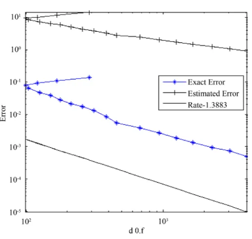
[image:6.595.185.449.303.428.2] [image:6.595.187.446.459.704.2]We report the results obtained for =10−2 and =10−4 over the domain Ω = −
(
1,1)
2.Figure 1 shows the successfully refined meshes created in the adaptive process for 2
10− =
, as well as the corresponding computed solution. Figure 2 shows the error curves for the exact and estimated errors. Figure 3
Figure 1. Adaptive grids (left) and solution (right) obtained for
2
10− =
& d.o.f:3663.
Figure 2. Estimated and exact error curves using 2
10− =
and Figure 4 show analogous results for the same problem with the parameter =10−4. The results show that the estimated error is well bounded as described in [22].
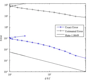
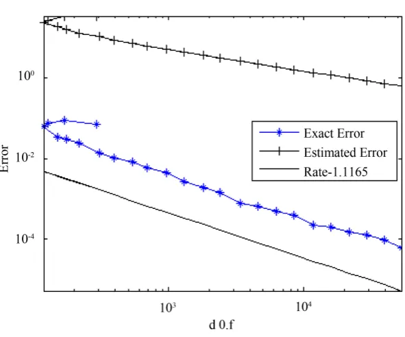
Example 2 (Interior layers) We consider Equation (2.1) with =10−2 and =10−4, b=
( )
2, 3T, Ω =( )
0,12. The forcing term f and boundary condition are determined from the exact solution:(
)
2 2 0.5 1
, 1
x y
u x y e
−
− + −
= +
[image:7.595.171.491.236.705.2] (4.2)
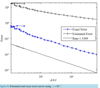
Figure 5 and Figure 6 clearly show that the adaptive method has successfully refined the correct elements using a greater concentration of elements in the interior layer. Figure 7 and Figure 8 show the estimated and exact error curves decrease monotonically for =10−2 and =10−4 respectively.
Example 3 (Interior and boundary layers) We consider Equation (2.1) with
T
π π
sin , cos
6 6
b= −
,
(
)
21,1
[image:7.595.176.454.283.411.2]Ω = − , f =0 and boundary conditions
Figure 3. Adaptive grids (left) and solution (right) obtained for 4
10− = &
d.o.f: 4183.
Figure 4. Estimated and exact error curves using 4
10− =
[image:7.595.176.455.446.705.2]Figure 5. Adaptive grids (left) and solution (right) obtained for 2
10− = &
d.o.f:5523.
Figure 6. Adaptive grids (left) and solution (right) obtained for 4
10− =
with
d.o.f:6259.
[image:8.595.168.464.454.700.2]Figure 8. Estimated and exact error curves using =10−4.
0 on 1 & 1,
1
tanh on 1,
1
tanh 1 on 1
2
x y
y
u x
x
y
= − =
−
= =
+ = −
(4.3)
Discontinuities at
( )
0,1 causes u to have an internal layer of width O( )
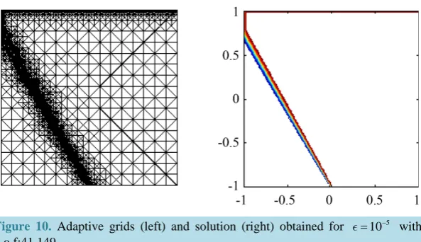
along the line y+ 3x= −1, with values u=0 to the left and u=1 to the right, as well as a boundary layer along the outflow boundary. We do not include error curves because no analytical solution is known in this case.Figure 9 and Figure 10 show some of the successively refined meshes created in the adaptive process for
3
10− =
and =105, as well as the corresponding computed solution. In the case of 2
10− =
in Example (2) and 3
10− =
in Example (3), the adaptive refinement process able to resolve the boundary and interior layers.
For the case of =10−4 in Example (2) and =105 in Example (3), it is hard to fully resolve the internal layers and the numerical solution display a small oscillatory pattern in the internal layer.
5. Conclusions
An adaptive finite element scheme for the convection-diffusion equation has been introduced and analyzed. This scheme is based on the Streamline Diffusion Finite element method combined with a Neumann-type error esti-mator.
Several numerical experiments are reported. For 3
10− ≥
, all of them show the effectiveness of this scheme to capture boundary and inner layers very sharply and without significant oscillations. But in the case of
4
10− =
in Example (2) and 5
10 =
Figure 9. Adaptive grids (left) and solution (right) obtained for =10−3 with
[image:10.595.166.463.265.436.2]d.o.f:34,897.
Figure 10. Adaptive grids (left) and solution (right) obtained for 5
10− =
with
d.o.f:41,149.
quite evident that our error estimator provides an effective refinement indicator even in the presence of internal layers.
References
[1] Hughes, T.J.R. and Brooks, A.N. (1979) A Multidimensional Upwind Scheme with no Crosswind Diffusion. In: Hughes, T.J.R, Ed., Finite Element Methods for Convection Dominated Flows, AMD, Vol. 34, ASME, New York, 19- 35.
[2] Hughes, T.J.R., Mallet, M. and Mizukami, A. (1986) A New Finite Element Formulation for Computational Fluid Dy-namics: II. Beyond SUPG. Computer Methods in Applied Mechanics and Engineering, 54, 341-355.
[3] Johnson, C., Nävert, U. and Pitkäranta, J. (1984) Finite Element Methods for Linear Hyperbolic Equations. Computer Methods in Applied Mechanics and Engineering, 45, 285-312.
[4] Roos, H.-G., Stynes, M. and Tobiska, L. (1996) Numerical Methods for Singularly Perturbed Differential Equations. Springer-Verlag, Berlin. http://dx.doi.org/10.1007/978-3-662-03206-0
[5] Johnson, C., Schatz, A.H. and Wahlbin, L.B. (1987) Crosswind Smear and Pointwise Errors in Streamline Diffusion Finite Element Methods. Mathematics of Computation, 49, 25-38.
http://dx.doi.org/10.1090/S0025-5718-1987-0890252-8
[6] Babuška, I., Durán, R. and Rodríguez, R. (1992) Analysis of the Efficiency of an a Posteriori Error Estimator for Li-near Triangular Finite Element. SIAM Journal on Numerical Analysis, 29, 947-964. http://dx.doi.org/10.1137/0729058 [7] Durán, R., Muschietti, M.A. and Rodríguez, R. (1991) On the Asymptotic Exactness of Error Estimators for Linear
Triangular Finite Elements. Numerische Mathematik, 59, 107-127. http://dx.doi.org/10.1007/BF01385773
[9] Babuška, I. and Rheinboldt, W.C. (1978) Error Estimates for Adaptive Finite Element Computations. SIAM Journal on Numerical Analysis, 15, 736-754. http://dx.doi.org/10.1137/0715049
[10] Bank, R.E. and Weiser, A. (1985) Some a Posteriori Error Estimators for Elliptic Partial Differential Equations. Ma-thematics of Computation, 44, 283-301. http://dx.doi.org/10.1090/S0025-5718-1985-0777265-X
[11] Ainsworth, M. and Babuška, I. (1999) Reliable and Roubst a Posteriori Error Estimation for Singular Perturbed Reac-tion-Diffusion Problems. SIAM Journal on Numerical Analysis, 36, 331-353.
http://dx.doi.org/10.1137/S003614299732187X
[12] Eriksson, K. and Johnson, C. (1993) Adaptive Streamline Diffusion Finite Element Methods for Stationary Convec-tion-Diffusion Problems. Mathematics of Computation, 60, 167-188.
http://dx.doi.org/10.1090/S0025-5718-1993-1149289-9
[13] Johnson, C. (1989) The Streamline Diffusion Finite Element Method for Compressible and Incompressible Fluid Flow.
Finite Elements in Fluids, 8, 75-95.
[14] Kay, D. and Silvester, D. (2001) The Reliability of Local Error Estimators for Convection Diffusion Equations. IMA Journal of Numerical Analysis, 21, 107-122. http://dx.doi.org/10.1093/imanum/21.1.107
[15] Verfȕrth, R. (1994) A Posteriori Error Estimation and Adaptive Mesh-Refinement Techniques. Journal of Computa-tional and Applied Mathematics, 50, 67-83.
[16] Verfȕrth, R. (1998) A Posteriori Error Estimators for Convection-Diffusion Equations. Numerical Mathematics, 80, 641-663. http://dx.doi.org/10.1007/s002110050381
[17] Almeida, R.C., Feijóo, R.A., Gale, A.C., Padra, C. and Silva, R.S. (2000) Adaptive Finite Element Computational Flu-id Dynamics Using an Anisotropic Error Estimator. Computer Methods in Applied Mechanics and Engineering, 182, 379-400. http://dx.doi.org/10.1016/S0045-7825(99)00200-5
[18] Peraire, J., Peiró, J. and Morgan, K. (1992) Adaptive Remeshing for Three-Dimentional Compressible Flow Computa-tions. Journal of Computational Physics, 103, 269-285. http://dx.doi.org/10.1016/0021-9991(92)90401-J
[19] Johnson, C. (1990) Adaptive Finite Element Methods for Diffusion and Convection Problems. Computer Methods in Applied Mechanics and Engineering, 82, 301-322. http://dx.doi.org/10.1016/0045-7825(90)90169-M
[20] Elman, H., Silvester, D. and Wathen, A. (2005) Finite Elements and Fast Iterative Solvers: With Applications in In-compressible Fluid Dynamics. Numerical Methods and Scientific Computation. Oxford University Press, Oxford.
[21] John, V. and Knobloch, P. (2007) On Spurious Oscillations at Layers Diminishing (SOLD) Methods for Convection- Diffusion Equations: Part I—A Review. Computer Methods in Applied Mechanics and Engineering, 196, 2197-2215. http://dx.doi.org/10.1016/j.cma.2006.11.013
[22] John, V. and Knobloch, P. (2008) On Spurious Oscillations at Layers Diminishing (SOLD) Methods for Convection- Diffusion Equations: Part II—Analysis for P1 and Q1 Finite Elements. Computer Methods in Applied Mechanics and
Engineering, 197, 1997-2014. http://dx.doi.org/10.1016/j.cma.2007.12.019
[23] Knobloch, P. (2007) On the Choice of the SUPG Parameter at Outflow Boundary Layers. Technical Report MATH-knm-2007/3, Charles University, Faculty of Mathematics and Physics, Prague.
[24] Eriksson, K., Estep, D., Hansbo, P. and Johnson, C. (1996) Computational Differential Equations. Cambridge Univer-sity Press, New York.
[25] Verfȕrth, R. (1996) A Review of a Posteriori Error Estimation and Adaptive Mesh-Refinement Techniques. Wiley- Teubner, Chichester.
[26] Ainsworth, M. and Oden, J. (1992) A Procedure for a Posteriori Error Estimation for h-p Finite Element Methods.
Computer Methods in Applied Mechanics and Engineering, 101, 73-96. http://dx.doi.org/10.1016/0045-7825(92)90016-D
[27] Papastavrou, A. and Verfȕrth, R. (2000) A Posteriori Error Estimators for Stationary Convection Diffusion Problems: A Computational Comparison. Computer Methods in Applied Mechanics and Engineering, 189, 449-462.
http://dx.doi.org/10.1016/S0045-7825(99)00301-1
[28] Chen, L. (2009) IFEM: An Innovative Finite Element Method Package in MATLAB. http://www.math.uci.edu/~chenlong/iFEM.html
[29] Chen, L. and Zhang, C.-S. (2008) AFEM@matlab: A MATLAB Package of Adaptive Finite Element Methods. Tech-nique Report, Department of Mathematics, University of Maryland College Park, College Park.
Submit or recommend next manuscript to SCIRP and we will provide best service for you: Accepting pre-submission inquiries through Email, Facebook, LinkedIn, Twitter, etc.
A wide selection of journals (inclusive of 9 subjects, more than 200 journals) Providing 24-hour high-quality service
User-friendly online submission system Fair and swift peer-review system
Efficient typesetting and proofreading procedure
Display of the result of downloads and visits, as well as the number of cited articles Maximum dissemination of your research work