vis c o-e l a s ti c fl ui d flo w t h r o u g h
c u r v e d pi p e s wi t h sli p e ff e c t s i n
p oly m e r flo w p r o c e s si n g
N o r o u zi, M , D a v o o di, M , B e g , OA a n d S h a m s h u d d i n , M D
h t t p :// dx. d oi.o r g / 1 0 . 1 0 0 7 / s 4 0 8 1 9-0 1 8-0 5 4 1-7
T i t l e
T h e o r e ti c al s t u d y of Ol d r o y d-b vis c o-e l a s ti c fl ui d flo w
t h r o u g h c u r v e d p i p e s wi t h sli p eff e c t s in p oly m e r flo w
p r o c e s si n g
A u t h o r s
N o r o u zi, M , D av o o di, M , B e g , OA a n d S h a m s h u d d i n , M D
Typ e
Ar ticl e
U RL
T hi s v e r si o n is a v ail a bl e a t :
h t t p :// u sir. s alfo r d . a c . u k /i d/ e p ri n t/ 4 7 8 6 2 /
P u b l i s h e d D a t e
2 0 1 8
U S IR is a d i gi t al c oll e c ti o n of t h e r e s e a r c h o u t p u t of t h e U n iv e r si ty of S alfo r d .
W h e r e c o p y ri g h t p e r m i t s , f ull t e x t m a t e r i al h el d i n t h e r e p o si t o r y is m a d e
f r e ely a v ail a bl e o nli n e a n d c a n b e r e a d , d o w nl o a d e d a n d c o pi e d fo r n o
n-c o m m e r n-ci al p r iv a t e s t u d y o r r e s e a r n-c h p u r p o s e s . Pl e a s e n-c h e n-c k t h e m a n u s n-c ri p t
fo r a n y f u r t h e r c o p y ri g h t r e s t r i c ti o n s .
INTERNATIONAL JOURNAL OF APPLIED AND COMPUTATIONAL MATHEMATICS
ISSN: 2349-5103 (Print) 2199-5796 (Online) Publisher: Springer
Accepted July 16
th2018
THEORETICAL STUDY OF OLDROYD-B VISCO-ELASTIC FLUID FLOW THROUGH CURVED PIPES WITH SLIP EFFECTS IN POLYMER FLOW PROCESSING
M. Norouzi1, M. Davoodi2, O. Anwar Bég3and MD. Shamshuddin4*
.1Mechanical Engineering Department, Shahrood University of Technology, Shahrood, Iran. 2. School of Engineering, University of Liverpool, Brownlow Hill, Liverpool, L69 3GH, UK.
3Aeronautical and Mechanical Engineering, Newton Building, University of Salford, Manchester, M54WT, UK. 4.Department of Mathematics, Vaagdevi College of Engineering, Warangal, Telangana, India.
*Corresponding author: [email protected]
ABSTRACT:The characteristics of the flow field of both viscous and viscoelastic fluids passing through a curved pipe with a Navier slip boundary condition have been investigated analytically in the present study. The Oldroyd-B constitutive equation is employed to simulate realistic transport of dilute polymeric solutions in curved channels. In order to linearize the momentum and constitutive equations, a perturbation method is used in which the ratio of radius of cross section to the radius of channel curvature is employed as the perturbation parameter. The intensity of secondary and main flows is mainly affected by the hoop stress and it is demonstrated in the present study that both the Weissenberg number (the ratio of elastic force to viscous force) and slip coefficient play major roles in determining the strengths of both flows. It is also shown that as a result of an increment in slip coefficient, the position of maximum velocity markedly migrates away from the pipe center towards the outer side of curvature. Furthermore, results corresponding to Navier slip scenarios exhibit non-uniform distributions in both the main and lateral components of velocity near the wall which can notably vary from the inner side of curvature to the outer side. The present solution is also important in polymeric flow processing systems because of experimental evidence indicating that the no-slip condition can fail for these flows, which is of relevance to chemical engineers.
KEYWORDS: Perturbation solution; Oldroyd-B fluid; Slip boundary-condition; Curved pipe; Weissenberg number;
Polymer dynamics.
PACS No. : 46.15.-X, 47.11. +j, 47.10. ab, 44.30. +v, 07.05. Tp.
1. INTRODUCTION
The significant diversity of engineering applications of the flow in curved pipes has grown in recent years and these so-called “Dean flows” have emerged in many complex areas of
biomedical engineering [1-5] and also chemical engineering [6-7]. Important investigations of
the flow in this regime were originally carried out by Dean [8-9] who used a theoretical
approximation and focused scientific attention on the effects of centrifugal acceleration (arising from the curvature of geometry) in the Navier-Stokes equations. Dean’s analytical
solutions were based on a perturbation method and highlighted most of the key features of
this regime such as Taylor-Görtler secondary flows, corroborating the previous empirical
investigation of Eustic [10]. Later studies by Topakoghlu [11] extended their work to the
perturbation solutions of both curved circular and annular conduits. Comprehensive reviews
of progress in these methods were presented by Berger [12] and later by Guan and Martonen
[13] and Naphon and Wongwises [14].
In all of the mentioned works the problem were solved subject to no slip boundary
condition. In recent years, slip flow investigations in micro-scale technologies are also
developed into an active arena of engineering sciences. Increasingly rich applications of such
flows are encountered in biophysical regimes, medical diagnosis, refrigeration systems,
chemical reactors, rocket thermal sciences and electronic component cooling mechanisms.
The ever-increasing desire for designing the highest performance small scale equipment has
led to considerable activity in experimental, analytical and numerical studies of microscale slip
flows. These studies principally concentrate on the effects of slip flow in the vicinity of the
boundary. This phenomenon generally plays a significant role in micro-scale related surveys of
Newtonian fluids. Earlier work by Hooman et al. [15] produced an analytical solution of flow
and heat transfer of an isothermal pipe in both hydrodynamically and thermally fully-developed
flow via a perturbation method. This analysis focused on the effects of slip flow and heat
transfer jump on gaseous flows with variable properties and showed that the presence of a slip
condition in micro scale geometries increases the flow rate and consequently heat transfer
rates. Contrarily, the temperature jump present around the contact surface of gas and solid
decreases the heat transfer value of this scenario. Both phenomena generally show a direct
relationship to the dimensionless parameter known as the Knudsen number in gaseous fluids,
this parameter is defining as the ratio of mean free molecular distance to an appropriate macro
length scale. Slip flows have been examined for a variety of different geometrical
configurations including conduits with different cross sections such as rectangular [16],
annular [17], hyper-elliptical and regular polygonal cross sections [18]. These studies have
also utilized the same slip flow and temperature jump conditions for Newtonian fluids.
In the past three decades, researchers have also directed substantial attention towards the
refined modelling industrially complex polymeric liquids with non-Newtonian formulations,
particularly viscoelastic fluids. Non-Newtonian transport in curved pipes has been a very active
area owing to a tremendous range of applications in polymer processing, biotechnology and
food stuffs, slurry transport, petrochemical treatment, pharmacological synthesis, heat
exchangers etc. The interesting influences of polymeric fluids related to the first and second
normal stresses [19-22] and relaxation and retardation characteristic times [23-27] on the flow
behavior and also heat transfer of these fluids has grown into a major field in its own right. An
extensive repertoire of analytical, numerical and empirical methods has been successfully
understanding of engineers. The collective influence of characteristics such as elastic force
and curvature of geometry and their important role in modifying Taylor-Gortler vortices also
make polymeric liquids a suitable potential choice for deploying even in small-scale
engineering mechanisms. In the non-slip case, Bowen et al. [28] implemented an approach similar to Topakoglu’s [11] to solve the full equations of motion for the creeping flow of upper-
convected Maxwell viscoelastic fluids. They also observed that viscoelasticity can generate a
pair of secondary flows in the same direction of rotation as that generated by inertial forces.
Ebadian [29] and Karahalios and Petrakis [30], using analytical approaches, tried to
investigate this issue and they all concluded that the first normal stress can generate a force
similar to hoop stress of inertial regime in Newtonian fluids, strengthening the secondary flow.
In a following work, Robertson and Muller [24] extended the model in [28] to a more general
case by considering viscoelastic inertial flow through circular and annular cross-section curved
pipes, reporting in detail the effects of Weissenberg and Reynolds numbers of this regime. In
the past, there were several reports in both macro and micro scales that polymeric fluids might
experience a slip phenomenon near the interface of the solid and the liquid that this issue can
also, potentially, be an important issue in the flow distribution of curved pipes. Hatzikiriakos
[31], in a review, discussed different types of slip occurring on molten fluids. In this work,
experimental evidences that molten polymers, slip macroscopically at solid surface is
reviewed. In following, different types of slip boundary condition is discussed and shown that
for some polymers even a second critical wall shear stress exists at which a transition to a
stronger slip regime occurs. Kaoullas and Georgiou [32] and Georgiou and Kaoullas [33],
showed that in the presence of slip yield stress both the classical no-slip boundary condition and an extension of the Navier’s slip phenomenon can be observed depending on the value of
the pressure gradient of Newtonian fluids. A similar behavior was observed for viscoelastic
Poiseuille flow with slip yield stress [34]. A more detailed study based on numerical and
analytical approach for linear and nonlinear Navier slip boundary conditions were carried out in
references [35-37].
Due to presence of secondary flow in curved pipe flow of viscoelastic fluids, these geometries
are of great importance in designing the highest performance cooling, mixing equipment etc.
Motivated by this issue, an important area which requires further analysis is the slip
hydrodynamics in proximity to the pipe (conduit) boundary. Therefore, in the present paper,
an analytical solution for laminar viscoelastic fluid moving through a curved channel is
developed to elucidate the effects of slip on flow characteristics. For this purpose, a
perturbation method is employed, in order to derive the closed form velocity field solutions up
to second order by considering the curvature ratio as the perturbation parameter. Analytical
approaches to viscous flows have been shown to be very powerful, as exemplified in recent
work by Siddiqui et al. [38] who employed Bessel and trigonometric functions to solve the
bi-harmonic equation arising in Stokes flow in narrow tubes with wall suction. In the current
work, the robust Oldroyd-B model is also implemented as the constitutive rheological
number, the Weissenberg number, the viscosity ratio and the slip coefficient on viscoelastic
flow in a curved channel are studied in detail. The present study provides a useful benchmark
for numerical and indeed experimental investigations of Dean Flows of viscoelastic fluids in
channels with wall slip and is of relevance to chemical polymer process engineering.
2. MATHEMATICAL FORMULATION
2.1 Dimensionless Group and Constitute Equations
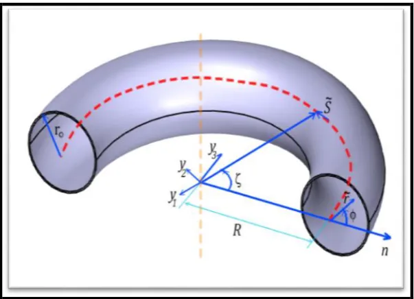
The physical configuration examined in the present study, namely slip flow of viscoelastic
fluids in curved channels is depicted in Fig. 1, where
r
0 and R are the cross-section radius and the pitch curvature radius, respectively. For the sake of convenience, it is conventional toemploy the dimensionless form of the momentum conservation equations. In line with this,
the appropriate non-dimensional variables and parameters implemented, are defined below:
0
0 0 0 0 0 0
0 0 0 1 0 0 0 0
0 0 0 0
.
.
.
,
,
,
,
,
,
,
,
,
,
,
r s
s s p p
v e
v e
v e
r
s
r
s
r
u
v
w
D
D
r
r
W
W
W
W
r
r
r
W
W r
r
P
P We
Re
W
W
W
r
R
=
=
=
=
=
=
=
=
=
=
=
=
(1)
where,
r
, φ ands
are the components of toroidal coordinate system.e
r,
e
ande
sare theunit vectors in these directions ,
r
0the radius of pipe,W0the maximum velocity of Newtonianfluid in terms of the pressure gradient of G(W0 =G r02/ 4),
v
the velocity vector,
sand
pthe solvent and polymeric parts of the stress tensor, Pthe pressure,1 the time constant offluid,the viscosity,Rethe Reynolds number,
the curvature ratio,R the curvature radius ofthe curved pipe,Dthe rate of deformation tensor and We the Weissenberg number. As
elaborated earlier, the robust, extensively studied, Oldroyd-B constitutive rheological equation
is employed to simulate the characteristics of the viscoelastic fluid. This model is also known
in the literature as a generalized Jeffreys model (Tripathi et al. [39] and Tripathi and Anwar
Bég [40]) and has also been implemented recently in gastric biofluid mechanics and polymer
pumping simulations. Essentially this model is derived by substituting the upper-convected
derivative with the time derivative of the Jeffreys model (due to its suitability in the simulation
of large deformation scenarios). The quasi-linear form of this model renders it more amenable
for analyzing the dynamics of dilute polymeric solutions. The Oldroyd-B model is presented
herein, based on Newtonian behavior for the solvent and the Upper-Convected Maxwell
(UCM) viscoelastic model for polymeric additives such that the
stress tensor of this modelFig. 1. The geometry of curved channel in current study.
s p
=
+
(2)
2 , 1 2 p
s p p
D D
s
= + = (3)
where
sis viscosity of Newtonian solvent and
pis viscosity of polymeric portions, respectively. The relationship between employed viscosity of the Oldroyd-B model and itscomponents can be expressed as:
s p
=
+
(4)In general form, the Oldroyd-B constitutive equation represents as [41]:
1
2 (D
2D
)
+
=
+
(5)where
1 is relaxation time,is rate of deformation tensor whichD
ime and is retardation t
2is the symmetric part of the velocity gradient. The components of the
D
tensor in therectangular coordinate system are defined as [41]:
1
(
)
2
i j
ij
i j
v
v
D
x
x
=
+
(6)The upper convected derivative of an arbitrary tensor
s
ij is defined as [41]:ij ij i j
ij k jk ik
k k k
s
s
v
v
s
v
s
s
t
x
x
x
=
+
−
−
(7)It is possible to show that if we define the stress of the Odroyd-B model as the summation of
UCM additive and Newtonian solvent stresses (Eq. (2)) then the retardation time constant can
be derived based on the viscosity ratio and relaxation time constant [41]:
2 1
p
=
(8)2.2 Governing Equations and Boundary Conditions
In the presented work, fully developed flow of polymeric solutions using the Oldroyd-B
constitutive equation is simulated. The Oldroyd-B model is a suitable choice for viscoelastic
materials showing a constant viscosity (Boger Fluids [42]). As it was reported in the literature
[31-37], the slip phenomenon can be observed in the interface of polymeric solutions and solid
interface. As we know, in the microfluidic devices (Microfluidics deals with the behaviour,
precise control and manipulation of fluids that are geometrically constrained to a small,
typically sub-millimetre scale [43-45]), the slip situation can more significantly influence in the
flow distribution of the material. In accordance with the Fig. 1, owing to the fully developed
situation, the derivatives of velocity components and the stress tensor with respect to the
angle of curvature (
) are assigned a zero value. The momentum conservation equations inthe
r
,
and s directions, for the steady fully-developed flow in a toroidal coordinate systemcan be represented as [23-24]:
(
) ( )
0 u r B v B
r
+ =
(9a)
2
1 1 1
2
cos [ ( )
Re
( cos sin cos )]
u v u v p rr r
u w rr
r r r B r r r r
rr r ss
B + − − = − + + + − + − − (9b)
1 1 1 2
2
sin [ Re
( cos sin sin )]
v v v vu p r
u w r
r r r B r r r r
ss r B + + + = − + + + + − + (9c)
1 1 1
( cos sin ) [ Re
2 ( cos sin )]
w v w p sr s
u w u v sr
r r B z r r r
rs s B + + − = − + + + + − (9d)
where,
B
designates the curvature radius of each point and is defined as:1
cos( )
The relations between lateral components of velocity and stream function of the secondary
flow are defined via Cauchy-Riemann equations, viz:
1
1
,
u
v
rB
B
r
= −
=
(11)Substituting the stream function from of Eq. (11) in Eq. (9a), automatically satisfies the
continuity relation. Also, the momentum equation in the pitch direction of curvature can be
expressed thus:
(
)
1 1 1 1
cos sin 4
2 cos sin
w w r s s
Re w r s
r r r r r r r r
r s s
− − + = + + + + + −
(12)In order to achieve possible solutions of velocity components it is necessary to eliminate
pressure gradient in the other directions of pipe except in the pitch direction which is already
identified. By reducing the derivative of Eq. (9b) and r derivative of equation (9c) from each
other, the equation in terms of stream function emerges as follows [23-24]:
2 2
2
2 2 2 2
2 2 2 3 2
2 2
2 2 3
1 1
2 sin cos
3 3 1 1
sin 2
3 1 3 2
cos
w w
Re w
r r r r r
r r r r r r r r r
r r r r r r r r
− + + + + − + + + − + + 2 2 2 2 2 22 2 2 2
2 2 2 2 2
sin 2 1 1
3 cos 2
2
1 1 1 1 3 1
1 1
sin
r r r r r r r
r
r r r r
r r r r r r r r r r
r
+ − − = − − + + + + − − +(
)
1 1 2
cos
s s r r
s s r r r
r
r r r
r r r r
− + − + − + − (13)
Therefore, the momentum equations are reduced into Equations (12) and (13) where
2denotes the Laplacian operator which is defined as:
2 2
2
2 2 2
1
1
r
r r
r
=
+
+
(14)It is customary that the slip coefficient would normally be taken to be the same for all
directions. In effect, the present approach decomposes the velocity vector into two
-subt (the tangential component) =
v t, where "t" is the vector tangent to the surface. This implies that fluid cannot flow through the wall but that the tangential velocity is proportional tothe tangential (shear) component of stress in the direction of flow. Considering the
above-mentioned description, the boundary condition for slip situation can be written as [46, 31-37]:
1 1 1
1
1
|
r v rs,
|
r v r,
|
r0
w
v
u
B
r
rB
= = =
=
=
=
= −
=
(15)where
vdenotes the slip coefficient between wall and fluid.3. PERTURBATION SOLUTIONS
Due to the quasi-linear, coupled nature of the momentum conservation equations and the
employed constitutive equation, a perturbation method is used to linearize the complex form of
these equations. The perturbation parameter in the momentum equations is considered to be
the curvature ratio (
=
r R
/
). So, in order for this expansion to have a wide range ofapplicability, it is necessary for any given geometry that the curvature ratio (
) be very small.However, according to previous studies this range can be a logical assumption in small scale
geometries [47-48]. Here,
=0 refers to the scenario of a straight pipe. Considering thequasi-linear form of the flow distribution in a straight pipe and consequently the absence of
secondary flow in this situation (
(0)=
0
), stream functions start from the first order onwards. The appropriate series forms for the stress tensor, stream function and main velocity are:( ) ( ) ( )
0 1 0
( , ),
( , ),
( , ),
n n n n n n
n n n
w
w
r
r
r
= = =
=
=
=
(16)3.1 Flow solution
Introducing series forms of the parameters defined in Eq. (16) into the momentum equation
(12) and arranging coefficients of
0, the first characteristic equation of the primary (main)velocity is obtained as:
4 2 (0) 2 (0) (0)
4 2 3
2
4
20
r
w
w
w
r
r
r
r
r
+
+
+
=
(17)The zero-order solution of the main velocity
w
(0) with respect to the slip condition around the wall (15) is:(0) 2
1
2
vw
= − +
r
(18) According to the rectilinear flow theorem of Longlois, Rivlin and Pipkin, the solution to thevelocity profile of viscoelastic fluids with a constant viscosity (Oldroyd-B fluids in our case) is
identical to the Newtonian fluids in rectilinear cases [41]. Although it should be noted that the
influence on the pressure distribution which is different than Newtonian cases. So, when the
value of
is equal to zero, the solution for velocity distribution is the same as the solution ofthe pipe flow of Newtonian fluids previously reported by Hooman et al. [15] for Newtonian fluid
in a straight channel with slip boundary condition. Also, in the case of no-slip,
v=
0
, theachieved solution (18) is identical to the no-slip velocity distribution of Newtonian fluid in
straight pipes. Arranging terms of order
1 in the Eq. (13), the first order characteristicequation of the stream function is obtained. The general solution of the characteristic equation
of
(1) is [23-24]:(1)
1
( )sin( )
g r
=
(19)Applying same method in Eq. (12), the characteristic equation of
w
(1) is obtained. The closed-form of the solution of this equation is derived as a function of the r parameter, multiplying witha cosine function as [23-24]:
(1)
1
( ) cos( )
w
=
f r
(20)Considering the Navier slip boundary condition near the wall (15),
g r
1( )
andf r
1( )
are calculated which is presented in the appendix with a more detailed information regarding thecalculation steps. After substituting the zero and first order velocity components and stress
tensors and utilizing the previous approaches for the second order of the main flow and
stream function, the characteristic equation of order 2 is obtained. Employing the
corresponding slip condition (15), the solutions of the characteristic equations of main flow and
stream function equations will be found. We consider the general forms of velocity
components as [23-24]:
(2)
2
( ) sin(2 )
g r
=
(21a)(2)
20
( )
22( ) cos(2 )
w
=
f
r
+
f
r
(21b)where
g r
2( )
,f
20( )
r
andf
22( )
r
are unknown functions which are laborious and for brevityare not presented, although they are considered in result
.
In this section, an analytical solution for the flow rate of Oldroyd-B fluids with slip present near
the wall of curved pipe is presented. The dimensionless flow rate through the pipe can be
simply presented as:
2 1
0 0
Q
w r dr d
=
(22)where w (axial velocity) is considered to be in the form of a perturbation expansion as:
(
)
(0) 2
1 20 22
( )
( ) cos
( )
( ) cos 2
w
=
w
r
+
f r
+
f
r
+
f
r
(23)Substituting the solutions of velocity components (which are achieved in previous part) into
Eqs. (22-23), the equation for the flow rate is obtained which due to the large size of the
equation is presented in the appendix.
4. RESULTS AND DISCUSSION
In this section, the derived analytical solutions are studied to explore combined effects of
slip coefficient, Reynolds and Weissenberg numbers, viscosity ratio and curvature ratio on
viscous and viscoelastic flows in curved channels. As it was previously reported in the
literature[31-37], the slip situation can occur in both micro and macro scale geometries for
polymeric solutions. To estimate a physical range of variable in the current problem, we refer
to the aqueous polymer solution used by Xu et. al. [49] with constant viscosity (=285 mPa.s).
This solution is prepared by adding 500 ppm (w/w) of a high-molecular-weight polymer (polyethylene oxide “PEO” of Mw= 4e06 g/mol) to a more concentrated 42.9% (w/w) aqueous
solution of the same polymer but of a much lower molecular weight (polyethylene glycol “PEG” Mw= 8000 g/mol) that provides a polymeric solution with relaxation time of 2.5 s and
density of 1080 (kg/m3). Depending on our choice of pressure gradient and the radios of the
pipe and the radios of the curvature, we can reach the range of variables which are used in
this section. Though, it should be noted, these variables are chosen as an example and one
can use the derived formula according to their geometry and rheological request.
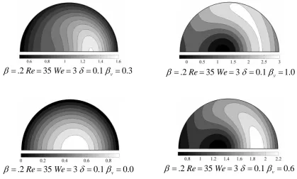
The flows of both Newtonian and Oldroyd-B fluids passing through straight pipes display the
well-known Poiseuille distribution. In this situation, the velocity contours of main flow are in
form of concentric circles (see Fig.2). An interesting phenomenon generated by centrifugal
force which causes these circles to deviate from the center line. Some typical sets of main flow
contours for Oldroyd-B fluids passing through curved channels are presented in Fig. 2. In this
paper, the flow results are presented only in half of the domain due to symmetric distributions
about the X-axis. In presented results, the left-hand side of the pipe represents inner side of
the curvature and the right-hand side corresponds to the outer side of the curvature. In this
figure, the first top four results are related to the classical Newtonian case. The data show that
in straight pipes even with the slip effect present, the flow distribution remains concentric. As
the wall shows non-zero constant patterns. The remarkable results in the Newtonian cases are
related to the scenario with slight curvature ratio of 0.1. It is evident that the flow distribution
around the wall is not constant anymore and can tangibly change along the wall.
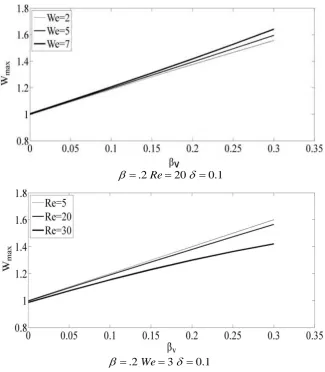
The presented data (Figs. 2 and 3) for viscoelastic cases also indicate that an increment in the
Reynolds number decreases the dimensionless maximum value of main velocity and causes
its position to deviate towards the outer side of the curvature. In contrast, the Weissenberg
number, the viscosity ratio and the curvature ratio are observed to enhance the maximum
value of main flow and progressively displace its position away from the center toward the
outer side of curvature.
0
v0.3(
Newtonian
)
=
=
35
0.1
v0.3(
)
Re
=
=
=
Newtonian
.3
Re
35
We
3
0.1
v0.0
=
=
=
=
=
.2
Re
35
We
5
0.1
v0.0
=
=
=
=
=
.2
Re
35
We
3
0.1
v0.2
=
=
=
=
=
=
0
v=
0(
Newtonian
)
35
0.1
v0(
)
Re
=
=
=
Newtonian
.2
Re
35
We
3
0.1
v0.0
.2
Re
45
We
3
0.1
v0.0
=
=
=
=
=
.2
Re
35
We
3
0.2
v0.0
[image:13.595.146.472.280.653.2]
=
=
=
=
=
Fig. 2. Distribution of the velocity (w) in different scenarios.
.2 Re 20 0.1
= =
=.2 We 3 0.1
20
3
0.1
Re
=
We
=
=
Fig. 3. Maximum value of the main component of the velocity versus the slip coefficient for different conditions.
Previously similar qualitative results were reported by Robertson and Muller [24] for the non-
slip situation. Another significant result is associated with the situation in which the flow
experiences slip (
v
0
). The present perturbation solutions show that in the slip situation, the maximum value of the main flow exceeds that obtained for the non-slip situation. Thereason of this phenomenon is related to the choice of the reference velocity which is made in a
way that the pressure gradient to be same as the equivalent Newtonian scenario with no slip
condition. So, if the pressure drop is fixed, in cases with slip we should expect the flow rate
and consequently maximum value of velocity to be increased (as it can also mathematically be
observed from equation (18))
Further results for the slip scenario as illustrated in Fig. 4 reveal that an increment in slip.
.2
Re
35
We
3
0.1
v0.3
=
=
=
=
=
.2
35
3
0.1
1.0
v
Re
We
=
=
=
=
=
.2
Re
35
We
3
0.1
v0.0
=
=
=
=
=
=
.2
Re
=
35
We
=
3
=
0.1
v=
0.6
[image:14.595.96.516.489.741.2]Coefficient causes the maximum value of velocity to migrate towards the outer side of
curvature. In these cases, velocity values vary from the outer side of curvature to the inner
side of curvature for non-zero curvature (
0
). However, the solutions at higher slip coefficient are qualitatively different. Some similar qualitative patterns of flow for the caseof
=0.2, Re=35, We=3,
=0.1 and
v=
0.6
were previously observed in high Reynolds number flows with no-slip by Robertson and Muller [24]. The data reveals howcuriously in high slip situations, the main flow may even show some recirculation phenomena.
According to the study of Mashelkar and Devaraja [50] hoop stress (
ss) in Newtonian cases is relatively weak and the pressure gradient in the core region of the pipe is balanced by thecentrifugal force. Fan et al. [22], based on an order-of-magnitude analysis for Oldroyd-B Dean
flows, derived an equation that estimates the relation between hoop stress (
ss) and centrifugal force. Considering the fact that lateral components of velocity are generallytwo-orders of magnitude smaller than the main velocity, the momentum equation in the "n"
direction of the pipe (see Fig. 1), far from wall and near the core region, can be reduced to:
2
Re
w
p
ssB
n
−
+
(24)The above equation simply implies that fluid inertia and hoop stress (
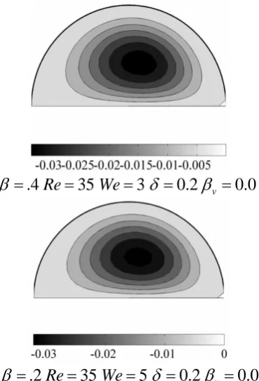
ss) are two significant and competitive forces near the core region which contribute to establishing the pressuregradient in "n" direction for Oldroyd-B fluids in pipes. Fig.5 depicts the hoop stress (
ss) contours for the different scenarios of non-slip and slip in both Newtonian and Oldroyd-Bfluids. As observed, the maximum value of the hoop stress in Newtonian case of Re=35 and
0.2
=
with non-slip is about 0.03. In the slip situation (
v=
0.2
), this value is 3 timesgreater than that for the non-slip regime. The hoop stress (
ss) value for Oldroyd-B fluid, with properties of (
=
0.2
andWe
=
3
), is found to be around 150 times higher than that computed for the Newtonian cases with slip (
v=
0.2
). In fact, this difference can even be enhanced 1400 times. Obviously, inertia force, near the wall and its vicinity, is weak (see Fig.2). Fig. 5 reveals that it is the relatively large axial normal stress near the wall which promotes
a secondary flow.
Non-Slip Newtonian Flow
(
v=
0)
=
.2
We
=
3
v=
0
Fig. 5. Contours of hoop stress (
ss) atRe
=
35
and =
0.2.
The direction of this secondary flow is observed to be in the same direction as that of the
inertial secondary flow. Considering the relationship between hoop stress and intensity of
secondary flows, it is estimated that increasing the slip should qualitatively offer a similar effect
as the Weissenberg number shows to enhance the intensity of the secondary flow.
.4
Re
35
We
3
0.2
v0.0
=
=
=
=
=
.2
Re
35
We
5
0.2
v0.0
=
=
=
=
=
.2
Re
35
We
3
0.2
v0.2
=
=
=
=
=
.2
Re
35
We
3
0.2
v0.0
.2
Re
35
We
3
0.3
v0.0
=
=
=
=
=
=
.2
Re
=
45
We
=
3
=
0.2
v=
0.0
Fig. 6. Secondary flow contours in different scenarios.
It is well known that flow in straight circular pipe shows rectilinear distribution without any
secondary flow in both non-Newtonian and Newtonian fluids. Fig. 6 depicts the secondary flow
shape of different fluids passing through a curved channel. These results confirm that an
increment in Weissenberg and Reynolds numbers and curvature and viscosity ratios
intensifies the secondary flows, a trend which has also previously been documented by
Robertson and Muller [24]. The present study has also shown that some significant and novel
results are related to the slip regimes. Fig. 7 shows that an increment in slip coefficient
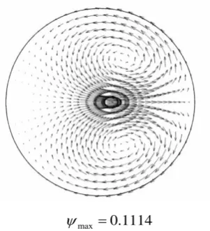
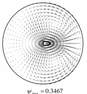
intensifies secondary flows.
max
0.1114
.2 Re 35 We 3 0.2 v 0.3
=
= = = = =
max
0.3909
.2 Re 35 We 3 0.2 v 1.0
=
[image:17.595.119.270.471.637.2]max
0.0299
.2 Re 35 We 3 0.2 v 0.0
=
= = = = = max 0.1799
.2 Re 35 We 3 0.2 v 0.5
=
[image:18.595.346.498.554.717.2]= = = = =
Fig. 7. Effect of slip coefficient on secondary flow and inducing second pair of vortices.
The data clearly demonstrate that the velocity distribution around the wall is not zero
(constant) any longer and markedly varies from the inside toward the outside of wall. As
previously presented in Fig. 4, the scenario with high slip situation can lead to the initiation of a
recirculation phenomenon.
Here, the solutions show that lateral components of velocity also change their own direction. It
appears that another pair of secondary flow in the opposite direction to the previous one is
produced. Fig. 8 reveals that an increment in other parameters can strengthen both secondary
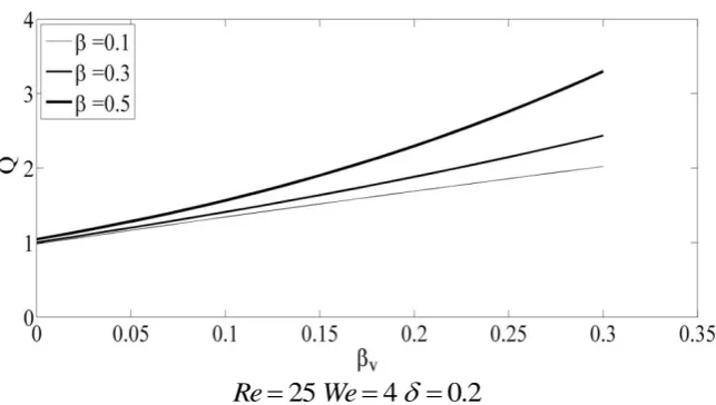
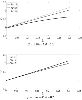
flows arising. Fig. 9 shows the flow rate of Oldroyd-B viscoelastic fluids in curved pipes and indicates that an increment in slip coefficient, viscosity ratio and Weissenberg number
enhances the flow rate whereas increasing the Reynolds number results in the converse effect
and decreases flow rate.
max
0.2313
.2 Re 35 We 5 0.2 v 0.6
=
= = = = = .2 45 max 0.34675 0.2 0.6
v
Re We
=
max
0.4039
.2 Re 35 We 5 0.3 v 0.6
=
= = = = =
max
0.0321
.2 Re 35 We 5 0.2 v 0
=
= = = = =
max
0.2997
.5 Re 35 We 5 0.2 v 0.6
=
= = = = =
max
0.2652
.2 Re 35 We 9 0.2 v 0.6
=
[image:19.595.148.470.559.741.2]= = = = =
Fig. 8. Mutual effects of different parameters on inducing second pair of vortices.
25
4
0.2
.1 We 5 0.2
= =
=.1 Re 45 0.2
= =
=Fig. 9. Dimensionless flow rate variation versus slip coefficient.
5 CONCLUSIONS
Analytical solutions have been derived using a perturbation technique, for the viscoelastic fluid
passing through a curved channel of circular cross-section, with a Navier slip boundary condition
present. A solution to the flow with slip boundary condition up to second order of the expansion
has been obtained to estimate characteristics of the flow regime. The Oldroyd-B rheological model
is employed due to suitability with liquids possessing constant stretch histories. The earlier
analysis of Fan et al. [22], proved that the flow characteristics of Oldroyd-B fluids in curved pipes
has a direct relationship with the hoop stress (
ss) component of the stress tensor. The present analytical results reveal that slip coefficient greatly effects the intensity and distribution of thisstress component, similar to Weissenberg number. A slight enhancement in the slip coefficient
between the wall and fluid can highly intensify the hoop stress. In the slip situation, a non-uniform
[image:20.595.147.472.69.464.2]curvature toward inside of the wall. Further analysis shows that an increment in Re, We,
and results in strengthening the secondary flows and causes the location of maximum velocity to
migrate towards the outside of curvature. The present solutions provide a useful benchmark for
numerical simulations and also experimental investigations related to Oldroyd-B viscoelastic flows
in curved channels. Future work will consider alternate viscoelastic models including the
Williamson [51] and Jeffery [52] models which also provide good approximations to polymer flows.
Acknowledgements
We express our gratitude to Professor Morton Denn of the Levich Institute, University of Delaware, USA, for his invaluable help and guidance regarding the present research. Furthermore, the authors acknowledge the comments of both reviewers which have served to improve the present article.
Compliance with Ethical Standards:
The ethical standards are considered in writing this paper. The authors have no conflict of interest
with anybody or any organizations/companies.
References
[1] W H Finlay, Phys. Fluids A1 854 (1989).
[2] T Hayat, S Noreen and A Alsaedi, J. Mech. Med. Biol. 12 1 (2012).
[3] M M Hoque, M M Alam, M Ferdows and O. Anwar Bég, Proc. Inst. Mech. Eng. H: J Eng. in Medicine227 1155 (2013).
[4] M Z Keshavarz and L Kadeem, Med. Eng. Phys.33 315 (2011).
[5] N Ali, M Sajid, Z Abbas and T Javed, Eur. J. Mech.-B: Fluids 29387 (2010). [6] V Kumar, M Agarwal and K D P Nigam, Chem. Eng. Sci.61 5742 (2006). [7] K C Cheng and M Akiyama, Appl. Sci. Res. 29 401 (1974).
[8] W R Dean, Phil. Mag. 4 208 (1927). [9] W R Dean, Phil. Mag. 5 673 (1928).
[10] J Eustice, Proc. Roy. Soc-London series A85 119 (1911). [11] H C Topakoglu, USSR J. Math. Mech.16 1321 (1967).
[12] S A Berger, L Talbot and L S Yao, Ann. Rev. Fluid Mech.15 461 (1983). [13] X Guan and T B Martonen, Aerosol. Sci. Tech. 26 485 (1997).
[14] P Naphon and S Wongwises, Renew. Sus. Energy Rev.10 463 (2006).
[15] K Hooman, F Hooman and M Famouri, Int. Commun. Heat Mass Transfer36 192 (2009). [16] W A Khan and M M Yovanovich, AIAA J. Thermophysics Heat Transfer 22 352 (2008). [17] Z Duan, Y S Muzychka, ASME J Heat Transfer130 1 (2008).
[18] A Tamayol and M Bahrami, ASME J Fluids Eng.132 1 (2010).
[19] M Norouzi, M Davoodi, O Anwar Bég and A A Joneidi, Int. J. Therm. Sci.69 61 (2013).
[20] M Norouzi, M H Kayhan, C Shu and M R H Nobari, J. Non-Newtonian Fluid Mech.165 323(2010). [21] M Norouzi, M Davoodi and O Anwar Bég, Int. J. Therm. Sci.90 90 (2015).
[22] Y Fan, R I Tanner, N Phan-Thien, J. Fluid Mech. 440 327 (2001).
[23] W Jitchote and A M Robertson, J. Non-Newtonian Fluid Mech. 90 91 (2000). [24] A M Robertson and S J Muller, Int. J. Non-linear Mech 31 3 (1996).
[25] C F Hsu and S V Patankar, AIChemE J. 28 610 (2004).
[29] M A Ebadian, ASME J. Appl. Mech. 57 1073 (1990).
[30] G T Karahalios and M A Petrakis, Acta Mechanica88 1 (1991). [31] S G Hatzikiriakos, Progress in Polymer Sci. 37(4) 624 (2012).
[32] G Kaoullas and G C Georgiou, J. Non-Newtonian Fluid Mech. 197 24 (2013). [33] G C Georgiou and G Kaoullas, Meccanica 48(10) 2577 (2013).
[34] Y Damianou, M Philippou, G Kaoullas and G C Georgiou, J. Non-Newtonian Fluid Mech. 203 24 (2014). [35] L L Ferrás, A M Afonso, M A Alves, J M Nóbrega and F T Pinho, J. Non-Newtonian Fluid Mech. 212 80 (2014). [36] L L Ferrás, J M Nóbrega and F T Pinho, J. Non-Newtonian Fluid Mech. 175 76 (2012).
[37] Y M Joshi and M M Denn, J. Non-Newtonian Fluid Mech. 114 185 (2003). [38] A.M. Siddiqui et al. Alexandria Engineering Journal, 56.1, 105 (2017).
[39] D Tripathi, O Anwar Bég and J Curiel-Sosa, Computer Methods In Biomech. Biomed. Eng. 17 433 (2014). [40] D Tripathi and O Anwar Bég, Int. J. Thermal Sci. 70 41 (2013).
[41] R B Bird and R C Armstrong, O Hassager and C F Curtiss, Dynamics of Polymeric liquids: Volume 1- Fluid Mechanics, New York: Wiley (1977).
[42] D F James, Annual Review of Fluid Mech.41 129 (2009).
[43] W M Abed, D W Richard, J C D David and J P Robert, Int. J. Heat and Mass Transfer88 790 (2015). [44] K Zografos, F Pimenta, M A Alves and M S N Oliveira, Biomicrofluidics 10(4) 043508 (2016).
[45] G K Satish, G Srinivas, D Li, C Stephane and R K Michael, Heat Transfer and Fluid Flow in Minichannels and Microchannels, Elsevier (2005).
[46] C L M H Navier, Mem. Acad. Sci. Inst. France 6 389 (1827).
[47] W M Abed, D W Richard, J C D David and J P Robert, J. Non-Newtonian Fluid Mech. 231 68 (2016). [48] W M Abed, D W Richard, J C D David and J P Robert, Int. J. Heat and Mass Transfer88 790 (2015). [49] H Xu, A Clarke, J P Rothstien and R J Poole, Appl. Phys. Lett. 108 241602 (2016).
APPENDIX
Due to the quasi-linear, coupled nature of the momentum conservation equations, a perturbation method is used. The perturbation parameter in the momentum equations is considered to be the
curvature ratio (
r
R
=
). Considering the rectilinear form of the flow distribution in a straight pipeand consequently the absence of secondary flow in this situation (
(0)=
0
), stream functions start from the first order onwards. The appropriate series forms for the stress tensor, stream function and main velocity are:( ) ( ) ( )
0 1 0
( , ),
( , ),
( , )
n n n n n n
n n n
w
w
r
r
r
= = =
=
=
=
(A-1)Introducing (A-1) into the momentum equation and arranging coefficients of
0, the first characteristic equation of the primary (main) velocity is obtained as:4 2 (0) 2 (0) (0)
4 2 3
2
4
20
r
w
w
w
r
r
r
r
r
+
+
+
=
(A-2) The zero-order solution of the main velocityw
(0) with respect to the slip condition around the wall is:(0) 2
1
2
vw
= − +
r
(A-3) Upon substituting Eq. (A-3) into the Oldroyd-B Constitutive Equation the zeroth order solution os the stress components can be calculated as:(0) (0) (0) (0)
(0) (0)
1
(0) 21
2,
,
2
((
)
(
) )
rs s ss
w
w
w
w
We
r
r
r
r
=
=
=
+
(A-4)After collecting the coefficient of
in Eqs. 17 and 16, the following equation can be obtained, respectively:2 (1) (1)
(0) 2 (1) 2 (1)
(0) (0)
2 2
2 (1) (1) 2 (1)
2 2 2
1
1
1
1
(2 Re
) sin
3
1
ss rr rr
r r r
w
w
r
r
r
r
r
r
r
r
r
r
r
r
−
= −
−
+
+
+
+
−
(A-5)(0) (1) 3 (0) (1) 2 (0) 2 (1) (0) (1)
2 (1)
3 2 2
(0) 3 (1) (0) 2 (1) (0) (1) (0) 3 (1)
2 2 3
1
1
4 cos
(
)
(
3
1
1
3
w
w
w
w
w
Re
We
r
r
r
r
r
r
r
w
w
w
w
r
r
r
r
r
r
r
r
=
−
−
−
+
−
+
−
−
(A-6)Using the perturbation series presented in eqn. (A-1) in constitutive equation, expressions for first order of stress tensor components can be obtained as:
(1) (1)
(1) (1)
2 (1) (1) 2 (1)
(1)
2 2 2
1
1
2
(
),
2
(
),
1
1
rr
r
r r
r r
r
r
r
= −
=
=
−
−
(A-7)Solution to the equation (A-5nad A-6), considering Eq. (A-7) will be in the form of
(1)
1
( ) sin
g r
1
5 5 5 7
(1 / 48) Re (1 / 12) (1 / 24) Re (1 / 288) Re (1 / 72) Re/(1 2 )
3 3 2
(1 / 9) Re/(1 2 ) (2 / 3) /(1 2 ) (1 / 3) Re/(1 2 )
2 (1 / 12) /(1 2 ) (1 / 2) . /(1 2 ) (1 / 4) Re/( (
1 2 )
(1 / )
32)
r r We r v r r v
r v v r vWe v r v v
rWe v r vWe v r v
g r v − − − + − + − + + + + + − + − + − + = +
3 3 3
Re/(1 2 ) (1 / 6) /(1 2 ) (3 / 16) Re/(1 2 )
r + v + r We + v + r v + v
(A-8)
5 2 2 7 2
(1920 /(23040 11520) 40 Re /(23040 11520)
5 2 2 2
320 Re /(23040 11520) (11 / 32) Re /(2 3 1)
5 5 2 2
640 Re/(23040 11520) 3840 /(23040 11520)
5
2560 Re /(23040 11
( )
1 r We v r v v
r v v r We v v v
r We v r vWe v
r W f e v r v + − + + + + + + = + + + + +
+ 520) 5760 3 Re /(23040 11520)
7 2 2 2 2
120 Re/(23040 11520) (5 / 3) /(2 3 1)
3 5 2
960 Re/(23040 11520) 30 Re /(23040 11520)
3 2 7 2
(5 / 6) Re/(2 3 1) 10 Re /(23040 11520)
(3 / 4) /
r We v v
r We v rWe v v v
r We v r v
rWe v v v r v
r − + − + − + + − + + + − + + − + −
2 3 2 2
(2 3 1) 4 /(2 3 1) (5 / 2) /
2 2 2
(2 3 1) (15 / 4) /(2 3 1) (19 / 11520) Re . /
2 3 9 2
(2 3 1) 8640 /(23040 11520) Re /(23040 11520)
3 2 3
40 Re /(23040 11520) 17280 /(23040 11520
r r
v v v v v v
r r
v v v v v
r r
v v v v
r v r v v
+ + + + + − + + − + + + + + + + + +
− + + + ) 320 3Re2 /
2 2 2 2 2
(23040 11520) (1/ 6) /(2 3 1) (127 /1920) Re /
2 2 2 2 3
(2 3 1) (209 /11520) Re /(2 3 1) (7 / 96) Re /
2 3 2 3 2 2
(2 3 1) 7680 Re /(23040 11520) 3840 /
(23040 11520
r v
rWe r
v v v v
r r
v v v v v v
r We r We E
v v v v
v − + + + + + + + + + + + + + − + −
+ ) 2 9Re2 /(23040 11520) 180 5Re2 /(23040 11520)
3 2 2 7 2 2
15360 /(23040 11520) 40 Re /(23040 11520)
2 2 2
(11/ 288) Re/(2 3 1) (77 /144) Re /(2 3 1)
3 2 2
720 Re /(23040 11520) (
r v v r v v
r We r
v v v v
r We r We
v v v v v
r v v
+ + + + − + − + + + + + + + −
+ + 7 / 6) 2 2/(2 2 3 1)
5 2 7
1920 Re /(23040 11520) 240 Re /(23040 11520)
r vWe v v
r We v v r We v v
+ +
+ + − +
(A-9)
The same method can be used to drive the characteristic equation of order 2 which due to large size of equations are not presented here but are included once results are reported. The solution to the characteristic equation of order two are in the forms of [23-24]:
(2)
2
( ) sin(2 )
g r
=
(A-10)(2)
20
( )
22( ) cos(2 )
w
=
f
r
+
f
r
(A-11)Solution of Flow Rate