Different Types of Fault Analysis and Techniques of Fault Location Using PSCAD

(1)

International Journal of Emerging Technology and Advanced Engineering

Website: www.ijetae.com (ISSN 2250-2459,ISO 9001:2008 Certified Journal, Volume 3, Issue 5, May 2013)

229

Different Types of Fault Analysis and Techniques of Fault

Location Using PSCAD

Heena Sharma

1

, M.T. Deshpande

2

, Rahul Pandey

3 1

M.E Student, Power System, SSTC, Junwani, Bhilai, CSVTU, Chhattisgarh, India 2_{Department of Electrical, SSTC, Junwani, Bhilai, CSVTU, Chhattisgarh, India}

3_{Department of Electrical & Electronics, SSTC, Junwani, Bhilai, CSVTU, Chhattisgarh, India}

Abstract— This Paper is Concentrated mainly to the

causes, Types and to locate the faults in cable. The paper presents different conditions of disturbances and faults in specified time period. In this paper there is a focus to solve the problem of location f fault which s used to prevent the unwanted outage, damage and failure of the cables. This paper also does the analysis about the voltage-time and current-time relationship during normal& different faulty condition. The proposed condition is evaluated by simulation using PSCAD software. It has been tested and found that the error of fault location is within ±5%.

Keywords—Cable, Fault, Fault location, PSCAD Software.

I. INTRODUCTION

In this paper an experimental study carried out an cable is presented. The aim is that to identify, locate and characterize the defect in the cables. The fault location methods are presented in this paper, along with utility statistics from a survey on cable fault location. Various case studies have been carried out including the different types of fault. The result obtained from the analysis will be useful in the development of a detect fault scheme for cable system in the future. Fault location in cable systems has existed since people first started installing power transfer equipment in the ground. On underground residential distribution cable systems, the cables will experience an increasing rate of failure as they near the end of their useful life. Many of the cable systems installed in the 1960s and early 1970s are now experiencing failures, and many are being replaced. These failures are causing problems for utilities, which must locate the faults. There are many fault location techniques at the disposal of utilities. There is a need for improving the speed of locating a fault, reducing the need for skilled operators, eliminating damage to the cable by the fault location equipment itself, and lowering equipment cost.

Terminal methods (e.g. the voltage drop ratio, capacitance method and the bridge technique) are applied to the cable from one or two terminals and are usually used for fault location. This paper is organized as follows. In section I, there was an introduction. In section II, an overview and description of Types of cable faults is presented. The simulation model and result of cable using PSCAD for grounded and ungrounded system is discussed in section III. A simulation model and Results of test methods on cable is presented and discussed in section IV. In section V, Result and conclusions are summarized.

II. TYPES OF CABLE FAULTS

For low voltage &medium voltage power cables the basic failure modes are:-

 Conductor short circuit to ground.

 Conductor to Conductor short circuit.

 Degraded insulation resistance.

 Open circuit.

Cable fault can be categorized into three main types :- Open conductor faults, shorted faults and high impedance faults.

a) Open-Conductor Faults: -In open-conductor fault,

the conductor of a cable is completely broken or interrupted at the location of the cable fault. It is possible to have a high resistance shunted fault (to ground) on one or both sides of the faulted conductor‟s location.

b) Shorted Faults: - A shorted fault is characterized

by a low resistance continuity path to ground (shunted fault).

c) High-Impedance Faults: - A high-impedance

(2)

International Journal of Emerging Technology and Advanced Engineering

230

III. SIMULATION MODEL AND RESULT OF CABLE USING

PSCADFOR GROUNDED AND UNGROUNDED SYSTEMS

Grounded System

1) Under normal condition:-

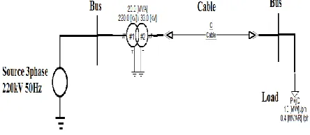
Here Three Phase 220 kV,50 Hz supply is given to the Three phase Two winding Transformer through Bus Bar and Three Phase Grounded system supplying the load through cable.

Fig. 1. Simulation Test Model of Three phase grounded system

supplying the load through cable during Normal Condition.

Fault Analysis:-

In This Source side graph, fault is not present so there is no distortion in waveform.

Main : Graphs

Time S 0.00 0.10 0.20 0.30 0.40 0.50 ...

... ... -30

-20 -10 0 10 20 30

V

o

lt

a

g

e

(

kV

)

[image:2.612.332.573.165.282.2]

Vsource_a Vsource_b Vsource_c

Fig.2 Source side three phase voltage graphs during normal condition.

In Load side graph is same as source side voltage graph because there is no fault.

Main : Graphs

Time S 0.00 0.10 0.20 0.30 0.40 0.50 ...

... ... -30

-20 -10 0 10 20 30

V

o

lt

a

g

e

(

kV

)

[image:2.612.55.277.257.354.2]

Vload_a Vload_b Vload_c

Fig.3. Load side three phase voltage graph during normal condition.

This is the waveform of Fault current,here fault current is zero because there is no fault in the circuit.

Main : Graphs

Time S _0.00 _0.10 _0.20 _0.30 _0.40 _0.50 ...

... ... -2.00

-1.50 -1.00 -0.50 0.00 0.50 1.00 1.50 2.00

F

a

u

lt

C

u

rr

e

n

t

(k

A

)

Ifa Ifb Ifc

Fig.4. - Fault current during normal condition.

2) Under Faulty Condition:-

[image:2.612.339.559.372.421.2]

Here Three Phase supply is given to the Three Phase two winding Transformer through 220 kV Bus Bar and Three Phase Grounded System Supplying the Load Through cable during Faulty Condition.

Fig.5. Simulation test model of Three Phase Grounded System supplying the Load through cable during faulty condition.

a)Single line to ground fault at distance 0.5km of 3km

three phase cable, applied at 0.2 second for duration 0.05 second (fault resistance is very low 0.01 ohm) Here, phase „a‟ to ground fault is shown in fig. voltage

sag in phase „a‟ is present.

Main : Graphs

Time S _0.00 _0.10 _0.20 _0.30 _0.40 _0.50 ...

... ... -30

-20 -10 0 10 20 30

V

o

lt

a

g

e

(

kV

)

Fig.6. Source side voltage graph during single line to ground fault

[image:2.612.61.284.428.538.2] [image:2.612.325.571.524.647.2] [image:2.612.47.296.585.699.2]

(3)

International Journal of Emerging Technology and Advanced Engineering

231

Main : Graphs

Time S _0.00 _0.10 _0.20 _0.30 _0.40 _0.50 ...

... ... -30

-20 -10 0 10 20 30

V

o

lt

a

g

e

(

kV

)

[image:3.612.320.578.119.258.2]

Fig.7. Load side voltage graph during single line to ground fault

Here distortion in waveform is present due to single line to ground fault and fault current in phase „a‟ increases due to low value of resistance.

Main : Graphs

Time S _0.00 _0.10 _0.20 _0.30 _0.40 _0.50 ...

... ... -4.0

-3.0 -2.0 -1.0 0.0 1.0 2.0 3.0 4.0 5.0 6.0 7.0

F

a

u

lt

C

u

rr

e

n

t

(k

A

)

[image:3.612.50.291.127.256.2]

Ifa Ifb Ifc

Fig.8. fault current during single line to ground fault.

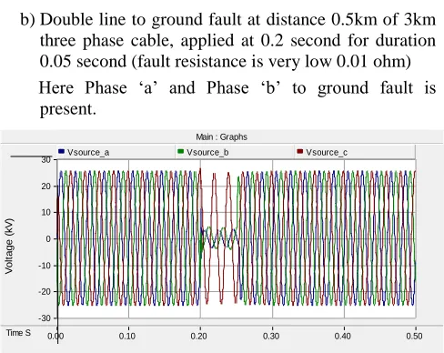
b)Double line to ground fault at distance 0.5km of 3km

three phase cable, applied at 0.2 second for duration 0.05 second (fault resistance is very low 0.01 ohm)

Here Phase „a‟ and Phase „b‟ to ground fault is present.

Main : Graphs

Time S 0.00 0.10 0.20 0.30 0.40 0.50 ...

... ... -30

-20 -10 0 10 20 30

V

o

lt

a

g

e

(

k

V

)

Fig.9. Source side voltage graph during double line to ground fault

Here, Voltage of Phase „a‟ and Phase „b‟ is zero due to double line to ground fault.

Main : Graphs

Time S _0.00 _0.10 _0.20 _0.30 _0.40 _0.50 ...

... ... -30

-20 -10 0 10 20 30

V

o

lt

a

g

e

(

kV

)

[image:3.612.324.565.307.437.2]

Fig.10. Load side voltage graph during double line to ground fault.

Here, Fault Current in Phase „a‟ and Phase „b‟ shown in fig.11

Main : Graphs

Time S _0.00 _0.10 _0.20 _0.30 _0.40 _0.50 ...

... ... -6.0

-4.0 -2.0 0.0 2.0 4.0 6.0 8.0

F

a

u

lt

C

u

rr

e

n

t

(k

A

)

[image:3.612.58.292.319.439.2]

Ifa Ifb Ifc

Fig.11. fault current during double line to ground fault

c)Three phase to ground fault at distance 0.5km of 3km

three phase cable, applied at 0.2 second for duration 0.05 second (fault resistance is very low 0.01 ohm) Here, Phase „a‟, Phase „b‟ and Phase „c‟ to ground

fault is present.

Main : Graphs

Time S 0.00 0.10 0.20 0.30 0.40 0.50 ...

... ... -30

-20 -10 0 10 20 30

V

o

lt

a

g

e

(

kV

)

Fig. 12. Source side voltage graph during three phase to ground fault

[image:3.612.48.292.454.648.2] [image:3.612.326.563.478.636.2]

(4)

International Journal of Emerging Technology and Advanced Engineering

232

Main : Graphs

Time S _0.00 _0.10 _0.20 _0.30 _0.40 _0.50 ...

... ... -30

-20 -10 0 10 20 30

V

o

lt

a

g

e

(

kV

)

[image:4.612.320.578.119.258.2]

Fig .13. Load side voltage graph during three phase to ground fault.

Here, Fault current in Phase „a‟, Phase „b‟ and Phase „c‟ is shown in fig14.

Main : Graphs

Time S 0.00 0.10 0.20 0.30 0.40 0.50 ...

... ... -6.0

-4.0 -2.0 0.0 2.0 4.0 6.0 8.0

F

a

u

lt

C

u

rr

e

n

t

(k

A

)

[image:4.612.48.297.125.256.2]

Ifa Ifb Ifc

Fig.14. Fault current during three phase to ground fault.

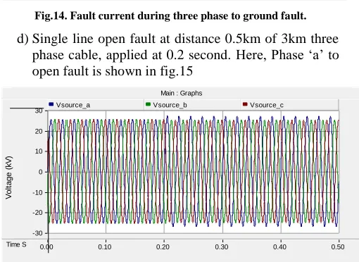
d)Single line open fault at distance 0.5km of 3km three

phase cable, applied at 0.2 second. Here, Phase „a‟ to open fault is shown in fig.15

Main : Graphs

Time S _0.00 _0.10 _0.20 _0.30 _0.40 _0.50 ...

... ... -30

-20 -10 0 10 20 30

V

o

lt

a

g

e

(

kV

)

Fig.15. Source side voltage graph during single line to open fault.

Here, Voltage of Phase „a‟ is zero due to single line to open fault.

Main : Graphs

Time S _0.00 _0.10 _0.20 _0.30 _0.40 _0.50 ...

... ... -30

-20 -10 0 10 20 30

V

o

lt

a

g

e

(

kV

)

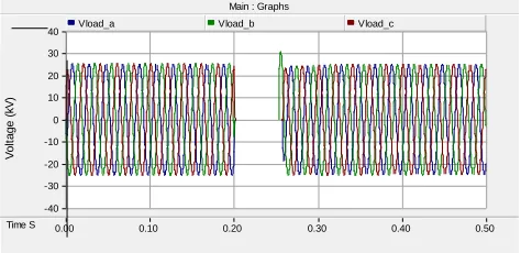
[image:4.612.49.293.309.428.2]

Fig. 16. Load side voltage graph during single line to open fault.

Here, Fault current is zero because single line to open fault.

Main : Graphs

Time S 0.00 0.10 0.20 0.30 0.40 0.50 ...

... ... -2.00

-1.50 -1.00 -0.50 0.00 0.50 1.00 1.50 2.00

F

a

u

lt

C

u

rr

e

n

t

(k

A

)

[image:4.612.324.575.310.438.2]

Ifa Ifb Ifc

Fig.17.Fault current during single line to open fault

Ungrounded System

1)Under normal condition:-

Here, Three Phase 220 kV, 50 Hz supply is given to the Three phase Two winding Transformer through Bus Bar and Three Phase Ungrounded system supplying the load through cable.

Fig.18 Simulation Test model for ungrounded cable system during normal condition.

Fault Analysis

[image:4.612.47.302.430.616.2] [image:4.612.325.557.542.598.2]

(5)

International Journal of Emerging Technology and Advanced Engineering

233

Main : Graphs

Time S 0.00 0.10 0.20 0.30 0.40 0.50 ...

... ... -30

-20 -10 0 10 20 30

V

o

lt

a

g

e

(

kV

)

Fig.19. Source side voltage graph during normal condition.

Here, Load side voltage graph is same as Source side voltage graph because there is no fault in circuit.

Main : Graphs

Time S 0.00 0.10 0.20 0.30 0.40 0.50 ...

... ... -30

-20 -10 0 10 20 30

V

o

lt

a

g

e

(

kV

)

Fig.20. Load side voltge graph during normal condition.

Here, Fault current is zero because there is fault is not present.

Main : Graphs

Time S _0.00 _0.10 _0.20 _0.30 _0.40 _0.50 ...

... ... -2.00

-1.50 -1.00 -0.50 0.00 0.50 1.00 1.50 2.00

F

a

u

lt

C

u

rr

e

n

t

(k

A

)

Ifa Ifb Ifc

Fig.21. fault current during normal condition.

2)Under Faulty Condition:-

Here Three Phase supply is given to the Three Phase two winding Transformer through 220 kV Bus Bar and Three Phase Ungrounded System Supplying the Load Through cable during Faulty Condition.

Fig.22. Simulation Test model for ungrounded system during faulty condition

a)Ungrounded system, Single line to ground fault at

distance 0.5km of 3km three phase cable, applied at 0.2 second for duration 0.05 second (fault resistance is very low 0.01 ohm)

Here, Phase „a‟ to ground fault for ungrounded system is shown in fig.23

Main : Graphs

Time S _0.00 _0.10 _0.20 _0.30 _0.40 _0.50 ...

... ... -50

-40 -30 -20 -10 0 10 20 30 40 50

V

o

lt

a

g

e

(

kV

)

Fig.23. source side voltage graph during single line to ground fault.

Here, Voltage of Phase „a‟ is zero due to single line to ground fault.

Main : Graphs

Time S _0.00 _0.10 _0.20 _0.30 _0.40 _0.50 ...

... ... -50

-40 -30 -20 -10 0 10 20 30 40 50

V

o

lt

a

g

e

(

k

V

)

Fig.24. Load side voltage graph during single line to ground fault.

(6)

International Journal of Emerging Technology and Advanced Engineering

234

Main : Graphs

Time S _0.00 _0.10 _0.20 _0.30 _0.40 _0.50 ...

... ... -2.00

-1.50 -1.00 -0.50 0.00 0.50 1.00 1.50 2.00

F

a

u

lt

C

u

rr

e

n

t

(k

A

)

[image:6.612.322.564.122.255.2]

Ifa Ifb Ifc

Fig.25. Fault current during single line to ground fault

b)Ungrounded system, Double line to ground fault at

[image:6.612.52.286.131.258.2]

Here, Phase „a‟ ,Phase „b‟ to ground fault is shown in fig. and phase of phase „a‟ and phase „b‟ are opposite due to Ungrounded system.

Main : Graphs

Time S _0.00 _0.10 _0.20 _0.30 _0.40 _0.50 ...

... ... -50

-40 -30 -20 -10 0 10 20 30 40 50

V

o

lt

a

g

e

(

kV

)

Fig.26. source side voltage graph during double line to ground fault.

Here, Voltage of Phase „a‟ and Phase „b‟ are zero due to double line to ground fault.

Main : Graphs

Time S 0.00 0.10 0.20 0.30 0.40 0.50 ...

... ... -50

-40 -30 -20 -10 0 10 20 30 40 50

V

o

lt

a

g

e

(

kV

)

Fig.27. Load side voltage graph during double line to ground fault.

Here, Fault Current in Phase ‟a‟ and Phase „b‟ are shown in fig.28

Main : Graphs

Time S 0.00 0.10 0.20 0.30 0.40 0.50 ...

... ... -6.0

-4.0 -2.0 0.0 2.0 4.0 6.0

F

a

u

lt

C

u

rr

e

n

t

(k

A

)

[image:6.612.48.297.325.490.2]

Ifa Ifb Ifc

Fig.28. Fault current during double line to ground fault.

c)Ungrounded system, three phase to ground fault at

Here, Phase‟a‟, Phase‟b‟ and Phase „c‟ to ground fault are shown in fig.29 and Phases of Phase „a‟, Phase „b‟ and Phase „c‟ are opposite due to Ungrounded system.

Main : Graphs

Time S 0.00 0.10 0.20 0.30 0.40 0.50 ...

... ... -30

-20 -10 0 10 20 30 40

V

o

lt

a

g

e

(

kV

)

Fig.29. source side voltage graph during three phases to ground fault.

Here, Phase ‟a‟, Phase ‟b‟ and Phase „c‟ voltage are zero due to three phase to ground fault.

Main : Graphs

Time S _0.00 _0.10 _0.20 _0.30 _0.40 _0.50 ...

... ... -40

-30 -20 -10 0 10 20 30 40

V

o

lt

a

g

e

(

kV

)

Fig.30. Load side voltage graph during three phase to ground fault

[image:6.612.325.564.343.481.2] [image:6.612.326.563.537.652.2] [image:6.612.56.298.546.662.2]

(7)

International Journal of Emerging Technology and Advanced Engineering

235

Main : Graphs

Time S 0.00 0.10 0.20 0.30 0.40 0.50 ...

... ... -8.0 -6.0 -4.0 -2.0 0.0 2.0 4.0 6.0 F a u lt C u rr e n t (k A )

Ifa Ifb Ifc

Fig.31.Fault current during three phase to ground fault

IV. SIMULATION MODEL AND RESULT OF TEST METHODS

ON CABLE

Terminal Fault Location Methods:-

1) Murray Loop: Murray loop test method is based on the principal of Wheatstone bridge technique, which is used a resistive bridge to determine the fault Location of cable. In the bridge, two variable resistors that are adjusted until the galvanometer G indicate null. Under this condition the bridge is balanced and the by the use of formula of distance to fault is used for fault Location in cable. This Method is valid for shorted, High impedance (shunt) fault and phase to phase fault on cable.

R =0 Vab V a b Vab V Main ... Galvanometer 0.00991753 Main ... Applied Volt... 24 0.50177899991 [ohm] 0.23888879999 [ohm] Eb Ea Ea Eb

Main : Controls Ea 14.8034 Eb 14.7935 Cable1 C C1Cable1 Cable1C1

Cable2 C C1_Cable2 _Cable2C1

0 .0 5 [o h m] Ea 1 Ea 2 Ea1 Ea2

Main : Controls Ea1

11.9612 Ea2

11.9513

Main : Graphs

0 10 20 30 40 50 ... ... ... -20.0 -15.0 -10.0 -5.0 0.0 5.0 10.0 15.0 20.0 y Ea1 Ea2

Fig.32. Simulation model of Murray loop test method for distance Location of faulty cable.

2)Charging current Method :- For Open Conductor Fault charging current Method is used in which a.c. voltage is applied between conductor and sheath of the faulty cable and determine the charging current I1 and rationed to the charging current of Un faulted cable I2 to determine the distance to fault in cable by formula. C1XLPE S1 C1 XLPE S1 XLPE C C1XLPE2 S1 XLPE2 C C1 XLPE2 S1 B1 B1 Timed Breaker Logic Closed@t0 Ica R=0 Ica 0 .0 1 [o h m]

cable Length charging current calculated cable (km) (amp) (km) 3.0km 0.0112597 3.0 1.0km 0.0044933 1.197 1.5km 0.00618416 1.64 2.0km 0.00787658 2.09 2.5km 0.00956119 2.54

Main : Graphs

Time S 0.00 0.10 0.20 0.30 0.40 0.50 ... ... ... -0.0150 -0.0100 -0.0050 0.0000 0.0050 0.0100 0.0150 C h a rg in g C u rr e n t Charging Current

Fig.33. Simulation Model of charging current method for distance Location of Faulty cable.

3)Voltage Drop Ratio Method:- For shorted and High

impedance(shunt) Fault and phase to phase to ground fault, voltage drop ratio method is used in which a constant d.c. current is applied to the faulted phase and to the Unfaulted phase with a jumper at the end of the cable.voltmeter is connected at faulted phase to ground or faulted phase to faulted phase, then two voltages can be determined and fault is locate by using formula. Cable1 C C1_Cable1 S1 C1 Cable1 S1 Cable2 C C1_Cable2 S1 C1 Cable2 S1 Ea 1 Ea 2 Ea1 Ea2

Main : Controls Eab 5.62716 Ea1 5.58643 Ea2 0.040723 Ia Ia Main ... Ia 0.05 Eab Eab

distance to fault = (Ea2/Eab)*length of cable d = (3.11935/ 9.44054)* 3km d = 0.99126km calculated fault distance

1.0km = d = 0.99126km 0.5km = d = 1.899km 1.5km = d = 1.499997km 2.0km = d= 2.0087km 2.99 km d = 2.968km

(8)

International Journal of Emerging Technology and Advanced Engineering

236

V. RESULT AND CONCLUSION

[image:8.612.315.570.181.456.2]

1) Result of Murray Loop Test Method.

Table 1.

Comparison between Actual and Calculated distance to fault in Murray Loop Test Method.

2) Result of Charging Current Method

Table2

Comparison between Actual and Calculated distance to fault in Charging Current Method

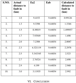
3) Result of Voltage drop ratio method

Table3

Comparison between Actual and Calculated distance to fault in Voltage drop ratio Method

S.NO. Actual distance to fault in (km)

Ea2 Eab Calculated distance to fault in (km)

1. 1.0 9.4153 9.44054 0.99126

2. 1.3 9.3398 9.44054 1.3346

3. 1.5 8.49019 9.44054 1.499957

4. 1.7 7.93949 9.44054 1.698

5. 2.0 7.2308 9.44054 2.0087

6. 2.3 6.321119 9.44054 2.2978

7. 2.5 5.343345 9.44054 2.523

8. 2.7 2.76324 9.44054 2.698

9. 2.9 4.199 9.44054 2.968

10. 3.0 3.11935 9.44054 2.992

VI. CONCLUSION

The simulation results show that the proposed method responds very well insensitive to fault type, fault Distance and system configuration. For the problem under consideration PSCAD simulation has been successfully applied. Therefore different types of fault analysis and fault location easily possible. Applied simulation methods are practically possible in field. Development for a wide range of cable length will be made in the further work in terms of safety and compact size for field measurements. Here different methods are used for different types of fault Location.

REFERENCES

[1] Hilary Marazzato, Ken Barber, Mark Jansen, Graeme Barnewall,“

Cable Condition Monitoring to Improve Reliability”, Asia pacific,2004.

[2] M.Villaran and R.Lofaro “Essential Elements of an Electric Cable

Condition Monitoring Program”, Brookhaven National Laboratorry, January 2010.

[3] Prof. Nelson chjumba,“High voltage cable insulation

systems”,2008.

[4] Matthias Boltze, Sacha,Michel Marklous, “On Line Partial

Discharge Monitoring & Diagnosis at Power Cables”, Annual International Double Client Conference,2009 .

S.NO. Actual

distance to fault in (km)

P (ohm) Q(ohm) Calculated

distance to fault in (km)

1. 1.0 0.41034 0.22517 1.0629

2. 1.3 0.38380 0.2735 1.2482

3. 1.5 0.3086 0.3586 1.6124

4. 1.7 0.2365 0.3293 1.746

5. 2.0 0.19335 0.3567 1.94545

6. 2.3 0.122413 0.43165 2.3379

7. 2.5 0.09972 0.46186 2.467288

8. 2.7 0.045811 0.4353 2.7143

9. 2.9 0.017299 0.50048 2.899

10. 3.0 0.0016781 0.50475 2.99

S.NO. Actual distance to

fault in (km)

Charging Current

Calculated distance to fault in (km)

1. 1.0 0.0044933 1.197

2. 1.3 0.0055 1.4

3. 1.5 0.00618416 1.64

4. 1.7 0.00686127 1.80

5. 2.0 0.00787658 2.09

6. 2.3 0.00889202 2.369

7. 2.5 0.00956119 2.54

8. 2.7 0.102406 2.728

9. 2.9 0.0109194 2.909

(9)

International Journal of Emerging Technology and Advanced Engineering

237

[5] A. Ngaopitakkul,C.Jettanson,C. Apisit and S.Jaikhan,

“ Identification Of Fault Location in Underground Distribution System Using Discrete Wavelet Transform” , IMECS,2010.

[6] El Sayed Tag El Din, Mohamed Mamdouh Abdel Aziz “An PMU

Double Ended Fault Location Scheme for Aged Power Cables” ,IEEE,2005.

[7] F.S. Nickel, T.M. Salas, D.E. Thomas, and C.M. Wiggins,

"Advanced Cable Fault Locator“, Final Report, EPRI EL-7451, October 1991, Electric Power Research Institute, Palo Alto, California.

[8] P.H. Reynolds, "Cable Fault Location Techniques“, Presented at the

Pennsylvania Electric Association Meeting, May, 197 1.

[9] E.C. Bascom, D.W. Von Dollen, “ Computerized Underground

Cable Fault Location ” , Expertise, IEEE 1994.

[10] V. Malathi and N.S. Marimuthu, Multi-class support vector machine

approach for fault classification in power transmission line, IEEE International Conference on Sustainable Energy Technologies (ICSET2008), pp. 67-71, 2008.

[11] Charles A. Maloney, "Locating Cable Faults", IEEE Transactions on

Industry Applications, Volume IA-9, No.4, July-August 1973.

[12] W. L. We2.9eks and J.P. Steiner, ”Instrumentation for the detection

and loca3.0tion of incipient fault on power cable,‟‟ IEEE Tran. On Power Apparatus and System, Vol. PAS-101, No. 7, July, 1982, pp. 2328-2335.

[13] I. Shim, J.J. Soraghan, and W.H. Siew, “Digital signal processing

applied to the detection of partial discharge: An overview,” IEEE Electrical Insulation Magazine, vol. 16, no.3, pp. 6-12, 2000.

[14] C. M. Wiggins, D. E. Thomas, T. M. Salas, F. S. Nickel, and H.

W.Ng, “A novel concept for URD cable fault location,” IEEE Trans.Power Delivery, vol. 9,no. 1, pp. 591–597, January 1995.

[15] S. Potivejkul, P. Kerdonfag, S. Jamnian and V. KinnaresN, “Design

of a low voltage cable fault detector,” Power Engineering Society Winter Meeting, 2000. IEEE , pp. 724-729 Vol. 1, 2000.

[16] E. C. Senger, G.Manassero, Jr., C. Goldemberg, and E. L. Pellini,

“Automated fault location system for primary distribution networks,” IEEE Trans. Power Del., vol. 20, no. 2, pt. 2, pp. 1332– 1340, Apr. 2005.

[17] M. S. Choi, S. J. Lee, D. S. Lee, and B. G. Jin, “A new fault location

algorithm using direct circuit analysis for distribution systems,” IEEE Trans. Power Del., vol. 19, no. 1, pp. 35–41, Jan. 2004.

[18] US NRC Generic Letter 2007-01, “Inaccessible or Underground