An Efficient Global Memory Addressing Technique for Beowulf Clusters Applied to Meshless Solutions of Maxwell’s Equations in Time Domain

(1)

International Journal of Emerging Technology and Advanced Engineering

Website: www.ijetae.com (ISSN 2250-2459, ISO 9001:2008 Certified Journal, Volume 7, Issue 4, April 2017)

149

An Efficient Global Memory Addressing Technique for

Beowulf Clusters Applied to Meshless Solutions of Maxwell’s

Equations in Time Domain

Elisson E. S. Andrade

1

, Rodrigo M. S. de Oliveira

2

, Marcelo B. S. Brandão

3

, Washington C. B. Sousa

4

,

Josivaldo S. Araújo

5

1,2,3,4,5_{Universidade Federal do Pará (UFPA) - Belém, Pará, Caixa Postal 8619, CEP 66073-900, Brazil.}

Abstract — Implementation of software for executing parallel simulations of problems in physics or engineering in computer clusters with distributed memory is usually complex because it involves the fragmentation of arrays and the passage of field information between different sub-domains. These processes can become extremely complex for numerical methods, especially for meshless approaches. In order to simplify the development of parallel programs, it is developed, implemented and validated a technique to unify memory addressing using application cache. With the proposed methodology, the basic structure of the original sequential code is preserved, dramatically simplifying the parallel implementation of numerical algorithms in parallel computer environments with distributed memory, such as Beowulf clusters.

Keywords — Application cache, Beowulf clusters, global memory addressing, meshless numerical methods, partial differential equations.

I. INTRODUCTION

The simulation of problems using computational electrodynamics methods is performed using numerical approaches to discretize Maxwell’s equations. Among the several existing methods, we have the finite-difference time-domain (FDTD) methods [1], the finite element methods (FEM) [2] and, more recently, the meshless methods (MM) [3]. However, the computational cost for obtaining numerical solutions of realistic problems can grow considerably when the following parameters are changed: discretization level, number of time steps and precision of the variables. As a result, the use of clusters for parallel processing becomes a valuable ally. However, it also pushes the responsibility of rewriting the algorithm for the parallel distributed memory architecture to the programmer [4].

Meshless methods are becoming more frequently applied to engineering problems [5][6] not only because of the absence of pre-defined meshes (which are complex to generate), but also because of the high level of geometric compliance to non-rectangular problems.

Besides, there is no need to solve, at each time step, linear systems of equations as it is demanded by FEM, for instance. However, the high demand for computational power, constantly present in scientific programming, stimulates researches for performance increases through the use of multiples computers and simplification of distributed memory handling. In these circumstances [7][8], the implementation of parallel applications becomes almost unavoidable if there is need for analysing complex (realistic) problems.

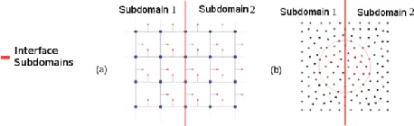
As previously mentioned, a major problem of using clusters in scientific problems treated numerically is the manipulation of data in distributed memory. In problems solved using FDTD methods, which is based on grids, the determination of interface cells in neighbour domains is predictable, since the points of the mesh are ordered in a structured way (Fig. 1(a)). However, in MM, there is no topological bond predefined among points, causing the determination of interface nodes of neighbour sub-domains to be specific for each case, making it difficult to obtain a generic solution for domain division in distributed memory environments [4], as it is illustrated by Fig. 1(b).

[image:1.612.331.560.596.666.2]

Recently, there was a significant progress in the process of making meshless methods parallel. Expressive increments of speedup have been obtained [7][8]. However, the developed techniques require manual adaptations of the sequential software to the cluster architecture, which reinforces the difficulty of generalizing parallelization of meshless methods in distributed memory systems.

Figure 1: Two-dimensional domain division into two sub-domains: (a) structured mesh and (b) meshless node set. Each subdomain is

(2)

International Journal of Emerging Technology and Advanced Engineering

150

In this paper, we present a new parallelization technique suitable for meshless methods. It is based on the use of application cache and on a global memory addressing schema over the cluster computers. The technique has a key contribution: drastically simplifies the parallelization of sequential algorithms. As a consequence, we have two additional benefits: the intrinsic reduction of processing time and automatic distributed memory allocation for problems that demands large computational resources. Notice that meshless methods can demand uneven memory use over the cluster nodes.

II. THEORETICAL BACKGROUND

Ampere-Maxwell and Faraday laws, in differential form, are given for dielectric, isotropic and non-dispersive media respectively by , = t E H      



(1) and , = t H E       



(2)

where H and E are the magnetic and electric field vectors, respectively,  is the electric permittivity of the medium,  is the magnetic permeability of the material and

t is time. In this paper, the analysis of the problem is performed using the transverse magnetic (TMz) mode. From (2), the components Hx and Hy can be obtained by solving the equations

          y E t

Hx z



1 = (3) and

,

1 =















x

E

t

H

y _z



(4)

respectively. From (1), one obtains

,

1 =

_

















y

H

x

H

t

E

z y _x



(5)

from which temporal integration provides Ez.

The RPIM method (radial point interpolation method) [3] is a meshless method, in which the value of a field component at a given node

x

is given by the interpolation of fields at points neighboring

x

.

The set of nodes

x

_h, which is used to determine a field component at

x

, is called support domain SR(x). Therefore, a scalar function

f

(

x

)

is approximated via the RPIM method by

),

(

)

(

=

)

(

)

(

1 = h h p n h a

x

f

x

f

x

f









(6)

Where np is the quantity of points in _SR(x),

f

(

x

)

is the value of

f

(

x

)

evaluated at

x

_h and



_h

(

x

)

is the value of the hth shape function at

x

associated to each

f

(

x

h

)

. It is possible to rewrite (6) as

, ) ( )

(x x F

f  (7)

Where F is the matrix with the field’s values

f

(

x

h

)

in each point

h

x of _SR(x) and  is the matrix of the np functions of form



_h.

As far as [3]

, ) , ( ) , ( F x y x x y x f       (8)

It is possible to approximate the spatial derivative in (3)-(5) using the RPIM method and the temporal derivatives using the centered finite difference technique. For example, the component Ez at a given point

x

is evaluated by

. ) ( ) ( ) ( = ) ( 1               



 y j H x j H t i E i

E Nt j

x p n j j t N y p n j t N z t N z    (9)

In (9), Nt is the index related to the current time step, given by Nt =t/t, where t is the time step, j is the index relative to the points

hj

x into the support domain and i is the index of the point

x

.

III. SEQUENTIAL ALGORITHM FOR RPIM

(3)

International Journal of Emerging Technology and Advanced Engineering

151

(a)

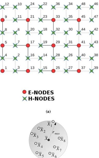
[image:3.612.75.266.144.448.2]

(b)

Figure 2: Meshless discretization of space: (a) the reference nodal arrangement in  (for rectangular discretization) adopted in this

paper and (b) support domain for x.

Each node has a computational index, as illustrated by Fig. 2a. This index is used to sort the nodes in RAM memory into a one-dimensional list Lp, in a way that all the nodes into Lp are juxtaposed in the memory. The representation of each node in the computer program is implemented by using a struct named node_RPIM. The properties of this struct can be seen in Table I.

In terms of temporal discretization, we have t = Ntt, where Nt=1,2,3,...,T/t. For satisfing the Courant-Friederichs-Lewy’s condition, it is adopted the value of t

as 99% of the limit imposed by this condition. It depends on the smaller distance between nodes arranged into 

Although the calculation of the electric and the magnetic fields are performed at the same computational instant Nt, the electric field is updated in the physical time t = Ntt and the magnetic field is updated in the physical instant t = Ntt+0.5t. Therefore, the simulation algorithm, for each discrete instant of time indexed by Nt must update all the nodes that represent the electric field (including the nodes with sources) and then update the fields at nodes where magnetic field is evaluated, completing a time step. The process is repeated until all the time instants in the interval of interest [0,T] are processed.

TABLE I

DEFINITION OF STRUCT NODE_RPIM

Property Description

x, y coordinates of

x

.

prop_EM Indicates whether the field calculated at

x

is electric or magnetic field.

P_Med Indicates whether the node is used as excitation source or as sensor.

Cx, Cy, Cz Components of E or H at

x

ds List with the indexes of the nodes in the support domain of

x

dphix, dphiy

Two lists with the values of the derivatives of the shape functions with respect to x and y, respectively, evaluated at

x

.

For performing the updates of electric field, it is defined the function calc_E(), which updated a component of E at all points in Lp using (9). The algorithm is given by (Fig. 3). The function calc_H() is dual to the function calc_E()

for the magnetic field. Calc_H is given by Fig.4.

(4)

International Journal of Emerging Technology and Advanced Engineering

[image:4.612.60.262.131.272.2]

152

Figure 4: Sequential algorithm for calculating Hcomponents in .

In addition, it was developed the function

calc_source_E(), that applies the excitation in nodes used as source. The function also writes on disk, at each time step, field values obtained in nodes used as sensors. The algorithm for this function is given by Fig. 5.

Figure 5: Implemented algorithm for field excitation on the nodes used as source in .

[image:4.612.324.561.551.629.2]

Finally, it is shown in Fig. 6 the sequential RPIM algorithm, which is used to solve Maxwell’s equations using the RPIM method with a single computer.

Figure 6: The sequential algorithm for the RPIM method.

IV. THE PROPOSED GLOBAL MEMORY ADDRESSING TECHNIQUE

The technique to simplify the use of unified memory addressing using application cache in meshless solutions, proposed in this work, aims to distribute the analysis domain among the memory of a computer cluster, but with global indexing to access the field data, keeping most of the sequential algorithm unchanged. This way, Ω is divided into sub-domains of approximately equal in size, in such a way that the data of each subdomain are stored in the memory of a distinct computer of the cluster. During the initialization of the program, each computer reads from a file on the hard drive mounted in the network exclusively the data of the nodes it will use. So, the list Lp, which stores all the nodes in the sequential code is divided, and each part of this division is properly stored in the memory of a distinct computer.

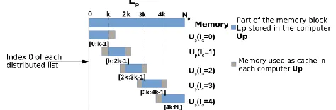
Therefore, each computer in the cluster will only calculate the field at the nodes stored in its own memory, reducing the total time of processing. However, a portion of the nodes of certain support domains that are close to the border will be stored in distinct computers, being necessary the data access of those data for performing calculation of fields (Fig. 1(b)). So, instead of requesting, at each temporal iteration, those data and transferring the information by explicit exchange of messages for each support domain close to the border between subdomains, we create areas of extra memory in each host, aiming at cloning data of nodes close to the borders, which are originally stored in neighbor computers. This process is illustrated by Fig. 7. It stands out that the area of extra memory, named as cache, do not impact in a significant way the use of local memory because the quantity of nodes being replicated is substantially inferior to the total quantity of nodes into the analysis region.

(5)

International Journal of Emerging Technology and Advanced Engineering

153

The list Lp is divided into smaller and continuous lists. However, in C/C++ the programmer can choose the access index of the first element in an ordered list, which is freely configurable [4]. Therefore, in our paralelization method, the nodes keep the same indexes used in the sequential case, even among the various computers of the cluster, facilitating the adaptation of the sequential code to be executed in parallel using the distributed memory system. To determine the number of nodes that each part of the list

Lp stores, we simply compute k = Np/nI, where k is the number of nodes stored into each computer, Np is the total number of nodes into Lp and nI is the number of instances being executed at the same time, which, in this paper, is equal to the number of computers in the cluster. From k, it is determined the interval of nodes that each computer stores. Two lists are created to store the interval of nodes that each computer works with: the list limitiInf stores the smallest index among the RPIM nodes at each computer and the list limitiSup stores the largest index among RPIM nodes stored by each cluster machine. Fig. 7 illustrates a list Lp distributed among various computers, maintaining the same access indexes of the sequential version of the RPIM algorithm.

By using the discretization method presented in [9], indexes of RPIM nodes can be tightly correlated to their spatial coordinates in most of the computational domain. Thus, the cache is usually needed only for the nodes stored locally into Lp and accessed with indexes smaller than those stored by limitiInf and/or larger than indexes stored by limitiSup. Therefore, to maintain the access to memory similar to the one used on the sequential code, the cache is settled up as indicated in Fig. 7 by the grayish memory sections of each computer Up (unity of processing). It worth noticing that the indexes of the nodes stored into the cache are identical to the indexes of the same nodes in the neighbor computers (that provided the data to the cache).

At each time advance of the simulation, we update the electric field E and, then, the magnetic field H according to the leapfrog time marching schema [1][9]. The field data in the cache are only updated after the update of the all the nodes outside of the caches associated to one given field (EorH). This way, it is possible to minimize the time used in the transmission of data via the Ethernet network. To perform the data exchange, we implement and use the function recieveCache() that, after identifying which field has just been updated (E or H), transfers only the data relative to that field to cache areas. Each instance of the code verify which other instance need to receive data calculated locally.

Next, the current instance sends the referred data to the proper Up, and subsequently waits for the receipt of field data of nodes updated by other instances. The wait ensures that the simulation is synchronized in all the computers involved. This is fundamental for preserving the leapfrog marching. The use of unsynchronized data in the field calculation in any node would produce physically inconsistent results, invalidating the proposed parallelization technique. The algorithm of the function

[image:5.612.333.553.482.627.2]

recieveCache() is given by Fig. 8.

Figure 8: Algorithm for performing data exchange for the current instance.

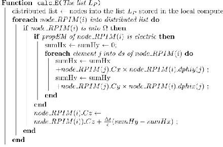
Because the field updates in each instance occurs exclusively in the nodes stored locally, with the proposed methodology it is needed to slightly modify the field update functions. This way, only the local part of the list Lp is visited by each computer. The algorithm of the function

calc_E(), modified to operate using the technique of unified memory addressing based on application cache for meshless solutions, is presented in Fig. 9.

Figure 9: Proposed algorithm for calculation of E in Ω subdomains.

(6)

International Journal of Emerging Technology and Advanced Engineering

154

Thus, the definition of the list of nodes to be processed by each computer and the correct cache initialization, along with the preservation of node indexes to be identical to the indexes produced for sequential processing, constitute the major modifications on the original RPIM algorithm. In conclusion, the final RPIM algorithm, parallelized by using the proposed technique and the developed sub-algorithms, can be seen in Fig. 10.

Figure 10: The Parallel RPIM algorithm based on technique of unified memory addressing based on application cache for meshless

solutions.

V. RESULTS

The proposed technique to simplify the use of distributed memory clusters based application cache is applied to obtain meshless solutions to Maxwell’s equations. Three specific cases were simulated to validate and to assess the performance of the parallelization technique. All the simulations were executed in a cluster of ten computers, which are interconnected by a Gigabit network. Each computer in the cluster has 8 GB DDR3 1 GHz RAM and is quipped with an Intel i5-3330 Quad-Core 3.0 GHz CPU.

A. Validation Case 1 - Free Space

The first simulation refers to the propagation of a plane wave in free space. In an analysis region with dimensions 80.05 m×60.05 m, the source, which is aligned parallel to the y-axis, was positioned at x = 3 m. The source is a Gaussian monocycle pulse given mathematically by

,

)

(

2 =

)

(

2

2 ) 0 (

0 2



t t

p

t

e

A

t

p

 



(10)

in which t is time in seconds, Ap is the pulse’s amplitude in V/m and



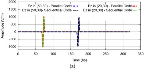
2001011s. The separation between nodes is given by 0.05 m (horizontally and vertically). The analysis region is discretized using 8031044 nodes and the total simulated time is T = 320 ns. It is used a time step of 20 ps to satisfy the Courant’s Condition.

[image:6.612.325.563.587.709.2]

For executing sequential and parallel simulations, two nodes are used as sensors positioned at (20,30)m and (50,30)m, respectively. The electric signals calculated during the entire simulation time at the referred nodes, in the parallel and sequential simulations, are compared in Fig. 11a. It can be seen that the data obtained sequentially and in parallel are perfectly coincident, validating the proposed parallelization method.

B. Validation Case 2 - RCS of a cylindrical scatterer

The second simulation performed deals with the calculation of the Radar Cross Section (RCS) [11, 12] of a cylindrical scatterer. The analysis region has dimensions 14 m×22 m. A massive metallic cylinder with radius of 1.5 m is surrounded by free space, where the center of the cylinder is placed at (8,11)m. The interior and surface of the cylinder are modeled with infinite electrical conductivity. Temporal and space discretization are the same as those used in Section V-A. However, due to the reduction of the analysis region (discretized with 585924 nodes), the simulated time was reduced to T = 80 ns.

Distributed around the cylinder, there are 264 sensors in which the field Ez is recorded for calculation of the RCS. The nodes are positioned equidistantly from the center of the cylinder (2 meter radius).

For calculation of the RCS, two simulations are needed: 1) a simulation with the cylinder inserted into free space, with which it is obtained the sum of the incident and reflected fields (total field) and 2) a simulation of free space only, without the cylinder, in which the incident field is calculated at the sensors [11]. Using the transient data obtained by each one of the 264 sensors, we have obtained the curves presented in the Fig. 11b. It can be seen that the results of the sequential simulation (Case 2) and parallel simulation (Case 3) are identical. The relative errors referring to the Cases 3 and 2 where calculated in relation to the Case 1 (the analytical result) and are shown in the

inset of Fig. 11b. The maximum absolute value of error is under 8.5%.

(7)

International Journal of Emerging Technology and Advanced Engineering

155

(b)

[image:7.612.49.288.131.393.2]

(c) (d)

Figure 11: Comparison between signals calculated in parallel and sequential simulations of a plane wave (a) in free space; (b) reflected by a metallic cylinder; (c) reflection coefficients and (d) transmission

coefficients obtained due to plane wave interaction with a PBG structure.

C. Validation Case 3 - PBG Filter

[image:7.612.47.288.542.687.2]

In the third case, we simulate the PBG filter illustrated by Fig. 12, which was originally analyzed in [9]. It consists on a three-layer infinite periodic structure composed of metallic cylinders. When a plane wave impinges on the periodic structure, well-determined frequency bands are allowed to pass through it, as illustrated by Fig. 11c.

Figure 12: Analysis region with a periodic structure: non-uniform discretization.

For performing the analysis, it was created an analysis region of 22 cm by 30 cm, with distance between nodes of 0.25 mm. The periodic structure is formed by 75 metallic cylinders arranged in 3 columns and 25 rows, with each metallic cylinder with a 0.5 mm radius. The centers of neighbor cylinders are distanced by 12 mm. The analysis region is discretized with 3293300 nodes. The discretization of analysis region can be seen in the Fig. 12. The plane wave, which is excited by a Gaussian monocycle pulse with 13

0 2250 10

  

t s and ₂₃₀₁₀13_{s, was} positioned at x = 2 cm, as it was arranged in [9].

The simulated time is T = 2.5 ns and the time step is 13

10 5 . 2   

_t s. Two nodes were used as electric field sensors: one for calculation of the transmission coefficient (Fig. 11d), at (0.18, 0.155)m, and another to calculation of the reflection coefficients, at (0.132, 0.155)m (Fig. 11c).

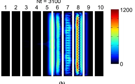
The propagation of the wave over the analysis region distributed among 10 computers (thus, ten sub-domains are used) can be seen in Fig. 13 for different time instants (Nt = 1100 and Nt = 3100). For the calculation of the transmission and reflection coefficients, two simulations had to be performed: one with a periodic structure and another in free space.

Using the calculated electric field at the sensor nodes, the reflection and transmission coefficients are computed. Results are shown by Figs. 11c and 11d, respectively, in which Case 4 refers to the results obtained with the sequential simulations, which are identical to the results of Case 5, obtained with parallel simulations.

(8)

International Journal of Emerging Technology and Advanced Engineering

156

[image:8.612.68.286.140.275.2]

(b)

Figure 13: Propagation of z-component of E through the periodic structure using the proposed parallelization technique at (a) Nt = 1100

and (b) Nt = 3100. Ten computers connected via Gigabit Ethernet are used: Ez can be seen in each sub-domain.

It can be seen that both results are close to results for Case 1, which is analytic [10], as well as to the results of the cases 2 and 3, which employ the Floquet boundary condition to simulate the structure with infinite length using FDTD and RPIM [9], respectively.

The results shown by Fig. s 11c and 11d validate the proposed parallelization method for complex structures.

D. Performance of the Proposed Parallelization Technique

By quantifying the processing time of each one of the RPIM simulations, using the serial program and parallel code in 2 to 10 networked CPUs, it is possible to measure the performance gain achieved by using the proposed technique. Time spent to calculate numerical solutions of the Maxwell’s equations is evaluated.

It can be seen in Table II that, for all cases, when the number of computers is increased, the processing time decreases, as expected. In ideal cases, the performance gain (speedup) [4] is equal to the number of processors used. However, because of the time spent in the transmission of data among the machines, there is always a reduced performance in comparison to the ideal case. The performance deviation  of the parallel simulation, taking as reference the ideal case, can be calculated by:

TABLE II

PROCESSING TIME FOR EACH SIMULATION

TABLE III

(9)

International Journal of Emerging Technology and Advanced Engineering

157

100%,

1 =

(%) 

    

  

    

  

 

I p

s

n t

t

 (11)

in which tp is the processing time of the parallel code and nI is the number of instances executed (equal to the number of computers used in the cluster).

Table III presents  for each performed simulation. It can be seen that for 4 CPUs or more the deviation  increases considerably with the reduction of the total number of nodes distributed on the analysis space. This can be justified by the fact that the processing time required by each machine to calculate field data, in each iteration, becomes closer to the time spent for the data exchange in the network. As a consequence, as the processing time gets closer to the time of required for network communication, the performance of the parallel software starts to present a high degree of dependence on the velocity of the transmission in the network used. Of course, the higher is the number of field nodes, the smaller is the rate of variation of  with respect to the number of CPUs, as it can also be seen in Table III.

VI. FINAL REMARKS

In this paper, it is proposed and implemented a technique for simplification of parallel programming in distributed memory clusters. The development of unified memory addressing technique based on application cache is the key concept established and implemented. After employing the technique for two-dimensional RPIM simulations, the performance deviation  is, at most, 30%. The results obtained with parallel processing are always identical to those obtained sequentially. Thus, it can be said that the developed method of parallelism is validated and that its performance is satisfactory for analysis of various electrodynamics problems solved with the RPIM method. The most important was achieved: parallel programming was drastically simplified, substantially reducing programming time as far as the final parallel program is virtually identical to the sequential code. This is achieved with special sub-algorithms developed and discussed in the present manuscript.

REFERENCES

[1] K. Yee, “Numerical solution of initial boundary value problems involving Maxwell’s equations in isotropic media,” Antennas and Propagation, IEEE Transactions on, vol. 14, no. 3, pp. 302–307, May 1966.

[2] M. N. Sadiku, Numerical Techniques in Electromagnetics, 2nd ed. , CRC Press LCC, 2011.

[3] J. G. Wang and G. R. Liu, “A point interpolation meshless method based on radial basis functions,” International Journal for Numerical Methods in Engineering, vol. 54, no. 11, pp. 1623–1648, 2002. [4] G. Andrews, Foundations of Multithreaded, Parallel, and Distributed

Programming, Addison Wesley, 2000.

[5] A. Afsari and M. Movahhedi, “An adaptive radial point interpolation meshless method for simulation of electromagnetic and optical fields,” Magnetics, IEEE Transactions on, vol. 50, no. 7, pp. 1–8, July 2014.

[6] Y. Tanaka, R. Tone, and Y. Fujimoto, “Study of an explicit meshless method using RPIM for electromagnetic fields,” Magnetics, IEEE Transactions on, vol. 49, no. 5, pp. 1577–1580, May 2013. [7] S. Ikuno, Y. Fujita, Y. Hirokawa, T. Itoh, S. Nakata, and A.

Kamitani, “Large-scale simulation of electromagnetic wave propagation using meshless time domain method with parallel processing,” Magnetics, IEEE Transactions on, vol. 49, no. 5, pp. 1613–1616, May 2013.

[8] S. Nakata, Y. Takeda, N. Fujita, and S. Ikuno, “Parallel algorithm for meshfree radial point interpolation method on graphics hardware,” Magnetics, IEEE Transactions on, vol. 47, no. 5, pp. 1206–1209, May 2011.

[9] W. C. B. Sousa and R. M. S. de Oliveira, “Coulomb’s law discretization method: a new methodology of spatial discretization for the radial point interpolation method,” Antennas and Propagation Magazine, IEEE, vol. 57, no. 2, pp. 277–293, April 2015.

[10] A. C. Tarot, S. Collardey, and K. Mahdjoubi, “Numerical studies of metallic PBG structures,” Progress In Electromagnetics Research, vol. 41, pp. 133–157, 2003.

[11] C. Balanis, Advanced Engineering Electromagnetics, Wiley, 2012. [12] K. Bavelis, “Finite-Element Time-Domain Modelling of Cylindrical