Application of Nonlinear Programming for Identification of Mathematical Models of Corrosive Destruction of Structures

(1)

International Journal of Emerging Technology and Advanced Engineering

Website: www.ijetae.com (ISSN 2250-2459, ISO 9001:2008 Certified Journal, Volume 6, Issue 11, November 2016)

86 Application of Nonlinear Programming for Identification of

Mathematical Models of Corrosive Destruction of Structures

George Filatov

Professor, Doctor of Techn. Sciences, Ukrainian State University of Chemical Technology, Ukraine

Abstract-- Considered the theorem on the belonging of optimal solutions one or more surfaces of the area permissible decisions. The results of investigations on the comparative evaluation of the identification of models of corrosive destruction with the help of analytical method and by random search method are presented.

Keywords-- Comparative Evaluation, Identification, Mathematical Models of Corrosive Destruction, Method of Least Squares, Random Search Method.

I. I

NTRODUCTION

Modern methods of calculation and design of chemical and petrochemical equipment require the use of mathematical models of corrosive destruction, allow to work off various options for the impact on the design of an aggressive environment, temperature, different load combinations, changing the properties of the material, etc. Analitical methods, used in computational practice for finding the extremum of optimized functions , for example, the method of least squares, are determine the extreme values of the control variables, regardless of the size of the area of permissible parameters. In the same case, if the area of permissible parameters has restrictions is limited, search of extreme control parameters is considerably complicated.

Existing mathematical models of corrosion destruction of structures interacting with aggressive media, as a rule, include a set of empirical coefficients whose values are determined by identifying the model to experimental data. On the region of existence of these factors usually are imposed restrictions: physical, geometrical, etc. It is possible that the extreme values of the coefficients belong to the boundary of permissible solutions. Let us investigate this issue in detail on the example of optimal designing of design.

II. THEOREM ON THE BELONGING OF OPTIMAL

SOLUTIONS ONE OR MORE SURFACES OF THE AREA

PERMISSIBLE DECISIONS

Consider the following theorem: At the optimal designing of structures the extreme value of the objective function belongs of one or of more surfaces of restrictions of the region of permissible parameters.

In the proof of the theorem, we'll refer to the manuscript work N.A. Alfutov and P.A. Zinovev "Some features of non-linear programming problems at the designing of structures of minimum weight", where the authors generalize the particular solutions given in [1], [7].

Let's formulate the problem of mathematical programming [3]:

minimize the function:

 

F



x

n



F

X



₁

,

₂

,...,

(1) at the performance of restrictions



n



j

x

b

g

₁

,

₂

,....,



,



,



, (2)

where:

X





x

₁

,

x

₂

,...,

x

_n



−

parameters. The problem (1) − (2) is a problem of nonlinear programming, if at least one of the functions

   

X

g

X

F

,

is non-linear.

Let's imagine the optimized structure as a set of discrete elements and denote the linear dimensions of discrete elements, taken as independent variables in the problem of nonlinear programming through xik, where

the subscript i denotes the number of the element, and

k

– the index of the linear dimension in the list of sizes, characterizing element i.

The objective function which expresses the weight or volume of the material of construction, consisting of discrete elements, in this case takes the following form:

 



_







i k ik

i

x

i

m

k

c

F

X

,

1 ,

2 ,...,

;

1 ,

2 ,

3

. (3)

Here: ci – the constant coefficients.

0 

ik

x

. (4)

Restrictions (4) have a geometric meaning and reduce the problem of mathematical programming towards the search of extremum function (1) which satisfy the restrictions (2), in a non-negative octant space

E

n

(2)

International Journal of Emerging Technology and Advanced Engineering

87

Consider the problem of nonlinear mathematical programming with inequality constraints:

 

b



j

m



g

_j

X



_j

,



1 ,

2 ,...,

(5) And let's investigate the function (2.3) in the extreme state. For this purpose, we use a generalization of the classical method of Lagrange multipliers in the case where the restrictions are given by inequalities. Transform the restrictions (5) in equalities. To do this, we introduce in the expression (5) auxiliary variables zj. We

get:

 

b

z



j

m



g

_j

X



_j



2_j



0 ;



1 ,

2 ,...,

. (6) As a result the conditions (5) are tantamount to inequalities:



j

m



z

2_j



0 ;



1 ,

2 ,...,

. (7)

The problem is reduced to the determination of the global minimum of the function

F

 

X

in a non-negative octant

E

nm. We form the Lagrangian:





 

_















m j j j j

j

g

b

z

F

z

1

2

,



X



X

(8)

where j – undetermined Lagrange multipliers.

Equating partial derivatives on





x

,

z

,





of upon all the variables, we obtain the following equation:





_

 

  

_















m j ik j j k i k i i ik

x

g

x

c

x

z

1 1 , 1 ,

0 ,

,

X



_

,

(9) −1 = 1,2 at k = 2,3; k− at k = 1; k + 1 = 2.3 when k = 1,2; k + 1 = 1 when k = 3:





0

2 ,

,

_

_

_







j j j

z



_

X

; (10)





_{ }

0 ,

,

_

_

2

_







j j j j

z

b

g

z

X



. (11)

Conditions (9) - (11) are performed in two cases. In the first of them all

z

_j



0 ,



_j



0

, which means that all the restrictions (6) are fulfilled as equations.

This case corresponds to the search for the minimum function F(X) in a non-negative octant space

E

m, at this the equality restrictions are not considered, since the system of equations (8) for



_j



0

has infinitely many solutions, belonging to a non-negative sites of coordinate axes of space

E

n, which as a rule does not satisfy the restrictions (5) and (11). In the second case the system of equations (9) − (11) has a solution if at least part

z

_j is zero. In this case the relevant restrictions (5) are satisfied with the equality sign.

In the geometric sense this assertion means that the

global minimum point of the function

F

 

X

in the presence of restrictions determined by the inequalities, belongs at least to one of the surfaces of restrictions.

This conclusion allows be recommended for finding of the extremum of nonlinear problems of mathematical programming the application of the zero-order methods that do not require the analysis of derivatives, for example, probabilistic methods.

Consider the example of the identification of one of the mathematical models of corrosion destruction. We formulate the task of identifying the mathematical model as a mathematical programming problem. As the object of the identification we take the logistic model of Verhulst (MMLV) [4].

)

exp(

1

₀ 0

t















, (12)

where



₀

,



,



–coefficients taking into account the effe



 the current value of the depth of corrosion damage;



₀ – upper limit of the depth of corrosion damage; t – time of corrosion.

Identification of the model is to determine the coefficients of the model



₀

,



,



, which would provide the best approximation of calculated curve described by equation (12), to the experimental curve. We write the expression for the objective function as functional: 2 1 0 0

)

exp(

1 





_



















n j j ej

t

J







. (13)

(3)

International Journal of Emerging Technology and Advanced Engineering

88

     

_

_

_

_

_

_

_

_

_

_

_

_

_

_



₀ ₀ ₀

;

,

(14) where



₀

,



₀

;





,





;





,



 the lower and upper limits of the values of the coefficients



₀

,



and



.

Introducing a vector of control variables



x

1

,

x

2

,....,

x

n





X

and denoting them









₀ ₂ ₃

1

,

x

,

x

, we obtain the following mathematical programming problem:

Find the minimum of the functional

2

1 2 3 1

1

)

exp(

1 min

)

(







_



















n j j эj

t

x

F

X



(15)

at the performance of restrictions:

0 )

(

;

0 )

(

;

0 )

(

;

0 )

(

;

0 )

(

;

0 )

(

3 3 6 3 3 5 2 2 4 2 2 3 1 1 2 1 1 1





































     

x

g

x

g

x

g

x

g

x

g

x

g

X

(16)

The formulated mathematical programming problem (15) − SGEF [5]. Restrictions on the area permitted by decisions taken by the following:

0 ,

01 



₀



5

mm;

0 ,

1000

0 ,

1 





;

0 ,

01 





10 ,

0

. The results of solution are shown in Table 1.

Таble 1

The results of the identification of the model MMLV of corrosive destruction by random search method

j

t

(years)

еj



(mm) 0



(mm)





(1/mm



year)

 

t

j



, mm



, %

0,1643 0,10

2,141 514,0 4,054

0,0179 +82,10

0,5753 0,49 0,4770 +2,65

1,0219 1,95 1,9966 -2,39

1,4410 2,10 2,1369 -1,60

2,0191 2,08 2,1410 -0,02

3,2000 2,25 2,1410 +4,84

Following are comparative assessments model identification MMLV and of some other models of corrosive destruction by random search method and by one of the analytical methods − by the least squares method.

III. COMPARATIVE ASSESSMENTS OF IDENTIFICATION

OF MATHEMATICAL MODELS OF CORROSION

DESTRUCTION BY THE ANALYTICAL METHOD AND

THE METHOD OF RANDOM SEARCH

To mathematical modeling of corrosion destruction of designs in recent years devoted a large number of publications [4, 6, 7, 8-10, 11].

As rightly pointed out in one of them [9], the construction of a mathematical model is to create a "...the aggregate of equations describing the deformation and the fracture of structures taking into account the mass transfer equations, of chemical interaction, of corrosive destruction and so on,. of the identification of these equations, i. e. the assessment of values of coefficients on the results of experiments, decision of the aggregate of equations and researching the behavior of structures. "

Consider the definition of the coefficients of the mathematical model of corrosive destruction at the external parameter of damage.

(4)

International Journal of Emerging Technology and Advanced Engineering

89

1) the fractional-linear model



t

T



t







₀

/



; (17)

2) the exponential model



t T



e

/

0

1







; (18)

3) mathematical model in the form of corrosive wear in view of logistical curve of Verhulst (MMLV):



t



e

0

1

0







_





(19)

Here:



₀  the maximum depth of corrosion damage;

T

 parameter of time;



,





(3); t time. In these models (17) − о,

T,



,



represent a sought coefficients.

To evaluate their in [4] is suggested by the method of least squares (LS) with the help of expression

 













n

j

j ej

t

J

1

2



, (20)

Where



_ej,



 

t

_j  respectively experimental and calculated parameter of damage in time t.

Table 2

The results of the calculation of rates of corrosion deterioration models by least squares (LS)[4] and by the random search method (RS)

Model

J

min



₀ (mm) t (years)





(1/mm year)

LS RS LS RS LS RS LS RS LS RS

Fractional-linear 2,362 0,713 2,371 3,553 0,218 1,409 - - - - Exponential

1,287 0,617 2,239 2,519 0,520 1,080 - - - - Logistical

0,501 0,026 2,250 2,141 - - 34,00 514,1 1,649 4,054 The coefficients of the model chosen, minimizing the

expression (20), we determine, equating the partial derivatives from the functional

J

over the values of 0,

T for models (17) and (18) and over the values of 0 ,



,



for the model (19). The result is a system of equations for determining the unknown coefficients.

However, the apparent simplicity of such approach is deceptive . Firstly, this system of equations is time-consuming and is complicated in the decision, for example, for an exponential model (18), and especially for the logistical model MMLV (19). Secondly, the coefficients, which were have been found by minimization of functional (20) by the method of least squares, not always correspond to the physical conditions of the problem. So, for example, in calculating the coefficients of a fractional-linear model (17) (Table 2) this model preliminary leads to linear form [4]

0

/



T



t

y





. (21)

Here:



t

y



.

The functional (20) takes the form:













n

j

ej

x

T

y

J

1

2 0

0

/



, (22)

where:

x

_j



t

_j

;

y

_e_j



t

_j

/



_e_j.

By minimizing the functional (22) over 1a

0



and

T/0 = b, we obtain the system of equations:



 

  









n

j

n

j j j

n

j

n

j

n

j j j j

j

y

bn

x

y

x

b

x

1 1

1 1 1

2

,

a

(23)

(5)

International Journal of Emerging Technology and Advanced Engineering

90  



 



 











































n j

j j n

j j

n j

j n

j j

y

x

n

y

x

n

x

1 1

1

1 2 2

1 0



;

_

















_

 

 n

j

n

j j

j

x

y

n

T

1 1

0

1



(24)

Calculation by the experimental data (Table 2) at number of observations

n



6

gives such values of parameters:



₀





357 ,

653

mm,

T





383 ,

528

years, that not corresponds to the physical conditions of task. At the same time are known [4] the quite real results:



₀



2 ,

3713

mm,

T



0 ,

218

years (Table 2.1.). Obviously, these results have been received not across the entire spectrum of experimental data, but only by part of it. If for determination of the coefficients we take observations № 3, 4, 5 and 6 (Table 2), i.e. on the upper portion of the experimental curve (Fig.1), the

model parameters



₀



2 ,

406

mm,

T



0 ,

2471

years are quite close to values adduced in [4].

A similar pattern occurs in the calculation of the coefficients for the exponential model (18). Parameters

0

[image:5.595.60.537.391.721.2]



and

T

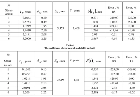
are determined on the points only № 3-but were extended to the whole range of observations. As a result, we get a big error on the initial stage of corrosive destruction, which reaches 506% for the exponential model (Table 4) and 920% for fractional-linear model (Table 3).

Table 3

The coefficients of fractional-linear model (RS method)

№

Obser-vations

t

j, years



ej, mm



0 , mm

Т, years

 

j

t



, mm

Error , % RS

Error, % LS 1 0,1643 0,10

3,553 1,409

0,371 -210,00 -920,00 2 0,5753 0,49 1,030 -110,20 -251,00 3 1,0219 1,95 1,494 +24,41 0,00 4 1,4410 2,10 1,796 +14,46 +1,90 5 2,0191 2,08 2,03 -0,61 -2,88 6 3,2000 2,25 2,467 -9,64 +1,33

Table 4

The coefficients of exponential model (RS method)

№ Obser-vations j

t

, years



_ej, mm



₀ , mm Т, years



 

t

, mm

Error , % RS

Error, % LS

1 0,1643 0,10

2,519 1,08

(6)

International Journal of Emerging Technology and Advanced Engineering

91

Analysis of the results of calculation of coefficients of fractional-linear model throughout the spectrum of observations allows us to conclude the feasibility of imposing restrictions on the area of permissible parameters in order to avoid getting physically incorrect data. Introduction of restrictions casts doubt on the applicability of the method of least squares to determine the coefficients selected mathematical model. The solution is offered to perform by one of the numerical methods of nonlinear programming − by random search method (RS).

In this case, the problem of mathematical programming is formulated as follows: find a minimum of the functional

 

















n

j

ej

t

j

n

J

1

2

,

1 ,



(25)

at the performance of restrictions:



x





q

s



g

_q



_i



_i

;

_i



_i



0 ,



1 ,

. (26)

Here:



 

t

_j  a function that takes the form (17) − (19);

x

_i  coefficients of mathematical models (17) − (19)



₀,

T

,



,



;

x

,

x

  accordingly the lower and upper limits of the sought coefficients.

[image:6.595.58.537.338.482.2]

The solution of the task is performed by the method of random search SGEF described in [5].

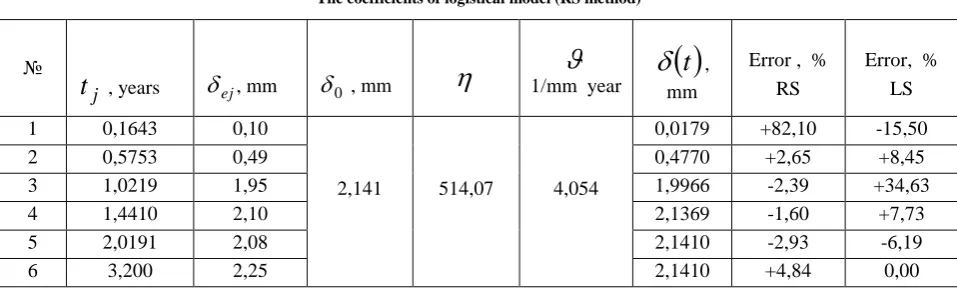
Table 5

The coefficients of logistical model (RS method)

№

j

t

, years



_ej, mm



₀ , mm





1/mm year

 

t



, mm

Error , % RS

Error, % LS 1 0,1643 0,10

2,141 514,07 4,054

0,0179 +82,10 -15,50 2 0,5753 0,49 0,4770 +2,65 +8,45 3 1,0219 1,95 1,9966 -2,39 +34,63 4 1,4410 2,10 2,1369 -1,60 +7,73 5 2,0191 2,08 2,1410 -2,93 -6,19 6 3,200 2,25 2,1410 +4,84 0,00

When calculating the coefficients of mathematical models (Tables 2−5) random search carried out under the following restrictions in the region permissible solutions:

5

01 ,

0 



₀



mm;

1 ,

0 





1000

,

0

;

0 ,

100

01 ,

0 





year

mm



1

.

Along with the coefficients of fractional-linear, exponential and models and MLKF model are defined error of calculated results compared with the experimental data. The low percentage of error calculated curves corresponding to the fractional-linear and exponential models [4], is explained because the method least squares operated only with the upper portion of experimental curve.

(7)

International Journal of Emerging Technology and Advanced Engineering

92

Fig.1. The graphs of fractional-linear model.

1 – experimental curve; 2 – calculated curve (method RS); 3 – calculated curve (method LS).

Fig.2. The graphs of exponential model.

1 – experimental curve; 2 – calculated curve (method RS); 3 – calculated curve (method LS).

Fig.3. The graphs of logistical model (MMLV).

(8)

International Journal of Emerging Technology and Advanced Engineering

93

Thus, the random search method proposed for estimation coefficients of mathematical models of corrosion damage is invariant to the type of model and allows to avoid serious mathematical difficulties encountered when using of determinative search methods, and provides solutions that enough accurately describe the actual processes of corrosive wear.

REFERENCES

[1] Gellatly, R.A. A procedure for automated minimum weight design. Part I./ R.A.Gellatly, R.H., Gallagher //Theoretical Basis. Aeron. Quart., 1966, v.7, №7, p. 63-66.

[2] Fіlatov, G.V. Optimal designing of constructions by random search method / − Dnipropetrovsk: UDHTU, 2003. − 433p. [3] Petrov, V.V.,.Ovchinnikov, I.G., Shihov, Yu.M. Calculation of

Structural Elements, Interacting with Aggressive Media / Saratov: Saratov State University. 1987. − 288 p.

[4] Karpunin, V.G. Study Bending and Stability of Plates and Shells Based on a Solid Corrosion [Text]: Author. Dis .... Cand. Tehn. Science / V.G Karpunin. − Sverdlovsk. 1977 − 24 p.

[5] Filatov, G.V. Random Search as the Method of Nonlinear Programming. Algorithms of Random Search / International Journal of Emerging Technology and Advanced Engineering, Volume 6, Issue 10, 2016, p.231-247.

[6] Gutman, E.M. Mechanochemistry metals and corrosion protection. M .: Metallurgy, 1974. 230.

[7] Ovchinnikov, IG On the methodology of structural models interacting with aggressive media // Durability of materials and structural components in aggressive and high temperature environments. Saratov: SPI, 1988. − P. 17-21.

[8] Ovchinnikov, I.G., Pochtman, Yu.M. Calculation and rational designing constructions exposed to corrosive wear (review) / FHMM. − 1991. − № 2. − p. 7-19.

[9] Ovchinnikov I.G., Sabitov, H.L. Modeling and prediction of corrosion processes / Saratov. 1982. − 61 p. − Dep. VINITI 16.03.82, № 1342.