BIROn - Birkbeck Institutional Research Online
King, Paul M. (1998) The free energy difference between 3-point water
models. Molecular Physics 94 (4), pp. 717-725. ISSN 0026-8976.
Downloaded from:
Usage Guidelines:
Please refer to usage guidelines at or alternatively
The Free Energy Differences Between 3-Point Water
Models
P. M. King
∗16 February 1998
Abstract
This paper describes precise calculations to determine the free energy differences between 3-point models of liquid water, using the method of thermodynamic integration and molecular dynamics. For the three models considered in this study the order of thermodynamic stability at 300 K and 1 atm pressure is SPC/E>SPC>TIP3P. The magnitudes of these stabilities are quantified and an estimate of the precision of the values is made.
1
Introduction
A number of models exist for the simulation of liquid water and aqueous solutions. The simplest models which adequately describe the structural, dynamic and thermodynamic properties of such systems are 3-point rigid models which interact only through Lennard-Jones and Coulombic interac-tions. In common use are the SPC,1SPC/E2and TIP3P3models, which find particularly widespread use in the solvation of biomolecular systems owing to their inclusion in widely used force-fields such as GROMOS4and AMBER.5 While the properties of these models have been widely investi-gated, to date there has been no precise calculation of the free energy differences between them. The purpose of the work reported in this paper is to make precise calculations of the difference in Gibbs free energy between these water models at 300 K and 1 atm pressure. Such calculations serve two purposes: Firstly, to analyze the suitability of the simulation protocol for determining what are antic-ipated to be relatively small absolute free energy differences, and secondly to provide an estimate of the free energy differences which will allow qualitative comparisons between results obtained from simulations using the different water models.
A number of authors have calculated free energy differences between various water models. Mezei6 has reported the excess Helmholtz free energy for SPC and other water models not considered in this study. The excess Helmholtz free energy of the CF7 and SPC models has also been computed using thermodynamic integration.8 Hermans9 has calculated the excess Helmholtz free energy of
∗Department of Chemistry, Birkbeck College, Gordon House, 29 Gordon Square, London WC1H 0PP, UK. Email:
SPC, SPC/E, TIP3P and TIP4P models of liquid water. These calculations used a relatively small number of molecules (80) which allowed for only a short non-bonded cutoff (6 ˚A). The excess free energy was determined using “slow growth”, coupling the water model of interest to an ideal gas of non-interacting molecules at the same volume, the change occuring in a period of 50 ps. The calculated values of the excess Helmholtz free energy of the 3-point models was calculated at -23.4, -26.8 and -22.6 kJ/mol for SPC, SPC/E and TIP3P respectively, indicating that SPC/E is the most stable model while the SPC model is marginally more stable than TIP3P. However, the precision of the calculations is difficult to determine using a slow growth procedure, and the quoted value of 0.4 kJ/mol is likely to be a lower bound. Heiner10 has considered the free energy differences between the models considered in this study. He evaluated the Helmholtz free energy difference between the models using a truncated taylor expansion of the free energy derivative, which involved simulating only a specific water model as a reference state.
2
Methods
For a classical system of N indistinguishable atoms in the isothermal-isobaric(N, p, T) ensemble the Gibbs free energy,G, at a pressurepand temperatureT is given by the expression11
G=−kBT ln ∆(N, p, T) (1)
HerekBis Boltzmann’s constant and∆(N, p, T)is the partition function,
∆(N, p, T) = 1
h3NN!
Z Z Z
exp −H(p,r) +pV kBT
!
dV dpdr (2)
his Planck’s constant andH(p,r)is the Hamiltonian of the system. The vectorsrandprepresent the position and momentum of all the atoms in the system respectively, andV is the system volume.
For all but the simplest systems it is not possible to determine the partition function. However, a number of methods exist for determining the free energy difference between two systems.12 The Hamiltonian of the system is made to depend on a coupling parameter,λ, such thatλ= λAdefines
the initial system, state A, andλ =λBdefines the final system, state B. Any intermediate state can be
chosen by specifying an intermediate value forλ. Issues relating to the choice of theλ-dependence of the Hamiltonian have been discussed at length,13although frequentlyλvaries between 0 and 1 as the system changes between states A and B, with the Hamiltonian having a linearλ-dependence,
H(p,r, λ) = (1−λ)H(p,r, λA) +λH(p,r, λB) (3)
It can be shown that the free energy difference is then given by the formula
=
Z λ=1
λ=0
*
∂H(p,r, λ)
∂λ
+
λ
dλ (4)
The termh. . .iλrepresents an ensemble average of the derivative of the Hamiltonian with respect to
λevaluated for a system defined byH(p,r, λ).
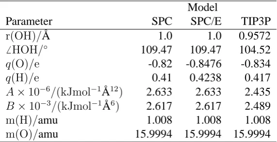
The water models considered in this study are the SPC and SPC/E models of Berendsen and co-workers,1, 2 and the TIP3P model of Jorgensen.3 In all three models the water molecule is considered as a 3-point rigid entity with an intermolecular interaction consisting of a Lennard-Jones 12-6 po-tential between oxygen atoms and a Coulombic term between all atoms, i.e.
VLJ =
O atoms
X
j>i A r12
ij
− B
r6
ij
(5)
VCoulomb =
all atoms
X
j>i
qiqj
4π0rij
(6)
whererij is the distance between atomsiandj on different molecules. The parameters for the three
water models are given in Table 1.
Model
Parameter SPC SPC/E TIP3P
r(OH)/A˚ 1.0 1.0 0.9572
6 HOH/◦ 109.47 109.47 104.52
q(O)/e -0.82 -0.8476 -0.834
q(H)/e 0.41 0.4238 0.417
A×10−6/(kJmol−1A˚12) 2.633 2.633 2.435
B×10−3/(kJmol−1A˚6) 2.617 2.617 2.489
m(H)/amu 1.008 1.008 1.008
[image:4.595.155.441.395.542.2]m(O)/amu 15.9994 15.9994 15.9994
Table 1: Parameters for water models
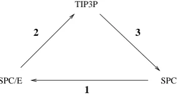
Free energy differences were determined from three transformations:
1 SPC(λ= 0)→SPC/E(λ= 1)
2 SPC/E(λ= 0)→TIP3P(λ= 1)
3 TIP3P(λ= 0)→SPC(λ= 1)
compared to 2.274 D for SPC. Transformations 2 and 3 involve changes in partial charges, geometry and Lennard-Jones interaction between oxygen atoms. In transformations 2 and 3 the changes in both geometry and Lennard-Jones interaction are equal in magnitude but are of opposite sign.
SPC
2 3
SPC/E
TIP3P
[image:5.595.211.389.137.231.2]1
Figure 1: Transformations performed between water models.
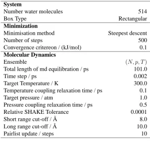
In each case the λ = 0 system was constructred and consisted of 514 molecules in a rectangular periodic box. This was then minimized for 500 steps using a steepest descent algorithm prior to being equilibrated using molecular dynamics for a period of 101 ps. During the molecular dynamics equilibration and the free energy determination the molecules were kept rigid by using the SHAKE algorithm14 thereby allowing a time-step of 0.002 ps to be used. Temperature and pressure were maintained using the weak-coupling scheme of Berendsen et al.15 Non-bonded interactions were evaluated at every step for molecules within a cutoff of 8 ˚A, while longer range non-bonded inter-actions were calculated every 10 steps for groups within 10 ˚A and kept constant between pair-list updates. The treatment of long-range interactions is an important issue in molecular simulation.16 While alternative schemes such as a reaction-field or an Ewald sum could have been incorporated, the relatively simple method used here was chosen as it is typical of methods used in biomolecular simulation. The system preparation conditions are summarised in Table 2.
For the determination of the free energy differences the derivative of the system Hamiltonian with respect to the coupling parameter was determined at six evenly spacedλ values; λ = 0.0, 0.2, 0.4, 0.6, 0.8 and 1.0. The value ofh∂H(p,r, λ)/∂λiλ was determined at eachλvalue by averaging over 50 ps (25000 steps) of MD simulation. For all simulations other than that at λ = 0.0 this period of averaging was preceded by a further period of 10 ps equilibration starting from an equilibrated configuration at the previous λ value. The protocol was such that reversibility in the free energy determination was very unlikely to be a problem, particularly given the small structural differences in the water models employed.
The derivatives required in Equation 4 are determined analytically for Lennard-Jones and Coulombic interactions. The contribution to the derivatives from the changes in geometry are also calculated analytically through use of the SHAKE procedure.4 There is no contribution to the derivative from kinetic terms as the masses of the atoms do not change during the course of the transformation.
System
Number water molecules 514
Box Type Rectangular
Minimization
Minimisation method Steepest descent
Number of steps 500
Convergence critereon / (kJ/mol) 0.1
Molecular Dynamics
Ensemble (N, p, T)
Total length of md equilibration / ps 101.0
Time step / ps 0.002
Target Temperature / K 300.0
Temperature coupling relaxation time / ps 0.1
Target pressure / atm 1.0
Pressure coupling relaxation time / ps 0.5
Relative SHAKE Tolerance 0.0001
Short range cut-off / ˚A 8.0
Long range cut-off / ˚A 10.0
[image:6.595.145.449.77.362.2]Pairlist update / steps 10
Table 2: Details of system preparation
3
Results and Discussion
For each of the transformations the averages of the calculated derivatives and associated errors over the entire 50 ps run are given in Tables 3, 4 and 5.
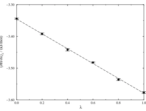
λ h∂Hp,r, λ)/∂λiλ/(kJ/mol)
0.0 -3.345±0.002
0.2 -3.392±0.003
0.4 -3.442±0.004
0.6 -3.482±0.002
0.8 -3.536±0.003
1.0 -3.577±0.003
Table 3: Averages for transformation 1.
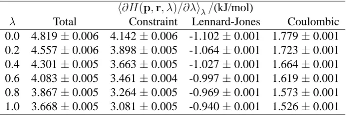
For transformations 2 and 3 the contributions to the total derivatives from the constituent terms are given. Owing to correlations in the data set used to determineh∂H/∂λiλ, the quoted precision in
the results was given as the standard deviation in the mean, calculated from Equation 74, 16
σ
"*
∂H ∂λ
+
λ
#
=
S
λ N
1/2
σ
"
∂H ∂λ
!
λ
#
h∂H(p,r, λ)/∂λiλ/(kJ/mol)
λ Total Constraint Lennard-Jones Coulombic
[image:7.595.121.478.78.196.2]0.0 4.819±0.006 4.142±0.006 -1.102±0.001 1.779±0.001 0.2 4.557±0.006 3.898±0.005 -1.064±0.001 1.723±0.001 0.4 4.301±0.005 3.663±0.005 -1.027±0.001 1.664±0.001 0.6 4.083±0.005 3.461±0.004 -0.997±0.001 1.619±0.001 0.8 3.867±0.005 3.264±0.005 -0.969±0.001 1.573±0.001 1.0 3.668±0.005 3.081±0.005 -0.940±0.001 1.526±0.001
Table 4: Contributions to averages for transformation 2
h∂H(p,r, λ)/∂λiλ/(kJ/mol)
λ Total Constraint Lennard-Jones Coulombic
0.0 -0.594±0.003 -3.079±0.004 0.939±0.001 1.545±0.001 0.2 -0.652±0.003 -3.159±0.004 0.937±0.001 1.570±0.001 0.4 -0.713±0.003 -3.248±0.004 0.938±0.001 1.598±0.001 0.6 -0.771±0.004 -3.330±0.005 0.936±0.001 1.624±0.001 0.8 -0.843±0.003 -3.433±0.003 0.937±0.001 1.653±0.001 1.0 -0.897±0.005 -3.521±0.005 0.939±0.001 1.685±0.001
Table 5: Contributions to averages for transformation 3
where σ[(∂H/∂λ)λ] is the square-root of the variance over an ensemble of size N, and Sλ is the
statistical inefficiency of the simulation. The procedure for calculatingSλ, based on the calculation
of sub-averages for different sized blocks of data, has been outlined elsewhere.16 The largest relative error on any value of the total derivative is approximately 0.6% — this is for transformation 3 where the value of the Hamiltonian derivative itself is much smaller than for the other two transforma-tions. In general the relative errors associated with all constituent term are approximately equal in magnitude and represent a high degree of precision.
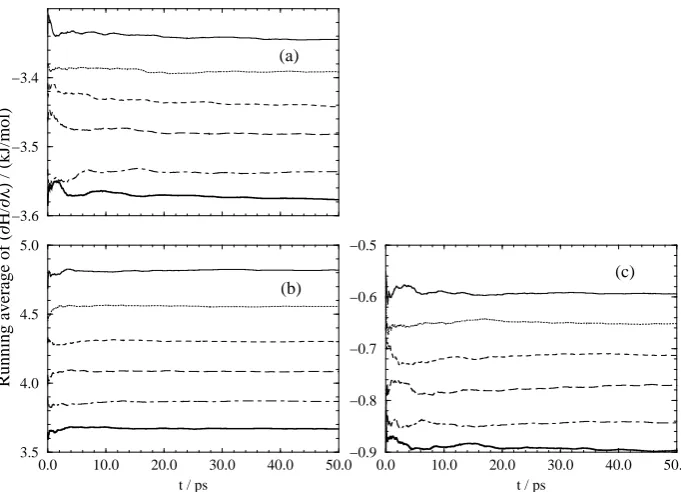
Figure 2 shows the running average of the total Hamiltonian derivative for each transformation.
For all the transformations the final average value is attained after approximately 20 ps of averaging. All the averages appear well converged after 50 ps of averaging with relatively little drift in the running average. The convergence of the average is better seen by calculating the relative deviation of the result as a function of time. Following Beutler et al.17 we calculate the relative deviation from the final free energy derivative at eachλvalue according to the following equation,
σsimrel(t) =
1− (1/t)
Rt
0G
0(t0)dt0
(1/tsim)
Rtsim
0 G0(t0)dt0
(8)
wheretsim represents the total simulation time, 50 ps, at a givenλvalue. In Figures 3, 4 and 5 the
0.0 10.0 20.0 30.0 40.0 50.0 t / ps
3.5 4.0 4.5 5.0 −3.6 −3.5 −3.4
0.0 10.0 20.0 30.0 40.0 50.0 t / ps
−0.9 −0.8 −0.7 −0.6 −0.5
(a)
(b) (c)
Running average of (
∂
H/
∂λ)
[image:8.595.124.465.90.336.2]/ (kJ/mol)
Figure 2: Running averages. The plots are (a) transformation 1; (b) transformation 2 and (c) trans-formation 3. In each plot the lines from top to bottom represent simulations atλ= 0.0, 0.2, 0.4, 0.6, 0.8 and 1.0 respectively.
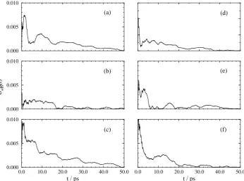
For transformations 1 and 2 σrel
sim(t) is below 0.5% within 10 ps of simulation, and in most cases
much sooner. For transformation 3σsimrel(t)is greater in magnitude since the error in the simulation results are of a similar value to those calculated for the other transformations yet the absolute value of the free energy difference is much less. However, even for transformation 3σrel
sim(t)is below 1.5%
within 20 ps.
Figures 6, 7 and 8 show the calculated derivatives as a function of the coupling parameterλ.
In each case there is a strong negative linear dependence between h∂H(p,r)/∂λiλ and λ. The
regression results are given in Table 6.
Slope / Intercept /
Transformation (kJ/mol) (kJ/mol) Correlation Value Error Value Error Coefficient 1 -0.234 0.004 -3.345 0.002 -0.9994
2 -1.149 0.031 4.790 0.019 -0.9985
3 -0.307 0.005 -0.592 0.003 -0.9995
Table 6: Summary of linear regression results
0.0 10.0 20.0 30.0 40.0 50.0
t / ps
0.000 0.005 0.010 0.000 0.005 0.010
σsim
(t)
0.000 0.005 0.010
0.0 10.0 20.0 30.0 40.0 50.0
t / ps (a)
(b)
(c)
(d)
(e)
(f)
[image:9.595.135.482.83.340.2]rel
Figure 3: Relative errors for transformation 1. The plots are (a)λ= 0.0; (b)λ= 0.2; (c)λ= 0.4; (d)
λ= 0.6; (e)λ= 0.8 and (f)λ= 1.0.
integration. The simulation error is estimated by taking the maximum error association with a given transformation,σmax, i.e.
Simulation error in∆G=±
Z 1
0
σmaxdλ
(9)
Table 7 shows the resulting free energy of each transformation.
Error
Transformation ∆G/ Integration / Simulation / Total / (kJ/mol) (kJ/mol) (kJ/mol) (kJ/mol)
1 -3.462 0.003 0.004 0.005
2 4.216 0.024 0.006 0.025
3 -0.746 0.004 0.005 0.006
Table 7: Free energy differencies calculated from linear regression
0.0 10.0 20.0 30.0 40.0 50.0
t / ps
0.000 0.005 0.010 0.000 0.005 0.010
σsim
(t)
0.000 0.005 0.010
0.0 10.0 20.0 30.0 40.0 50.0
t / ps (a)
(b)
(c)
(d)
(e)
(f)
[image:10.595.133.481.82.341.2]rel
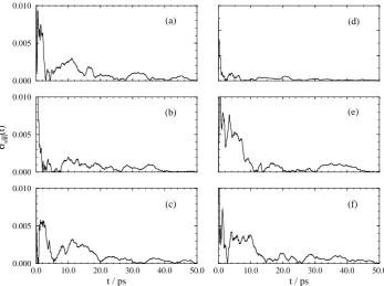
Figure 4: Relative errors for transformation 2. For key see Figure 3.
the correlation coefficient for quadratic regression of the total derivatives is 0.9999.) However, integrating the result does not significantly affect the calculated free energy difference, so the linear regression results are quoted and provide an upper bound for the integration errors.
For transformations 2 and 3 it is possible to separately consider each of the terms contributing to the overall derivative of the Hamiltonian and these are reported in Table 8. The only contribution which does not give a precise result on regression is the Lennard-Jones contribution for transformation 3. Here the derivative is effectively constant and the error associated with integration is similar whether one uses analytical or numerical integration. The sum of each term around the cycle should be zero. It can clearly be seen than the Gibbs free energy difference around the cycle, at (0.008 ±0.026)
kJ/mol, is effectively zero to within about ±0.03 kJ/mol. For the individual components of the free energy it is evident that around the cycle they do not sum to zero. This is in accord with the realization that while the total free energy of a system is a state function, its components are not well-defined quantities in that they are path dependent.13, 18–20 For example, from Table 8 it can be seen that the constraint terms in transformations 2 and 3, which one might anticipate to be of equal magnitude but opposite sign, differ by a significant amount. Only when the energy terms relate to independent coordinates will the components be path independent.
0.0 10.0 20.0 30.0 40.0 50.0
t / ps
0.000 0.015 0.030 0.045 0.000 0.015 0.030 0.045
σsim
(t)
0.000 0.015 0.030 0.045
0.0 10.0 20.0 30.0 40.0 50.0
t / ps (a)
(b)
(c)
(d)
(e)
(f)
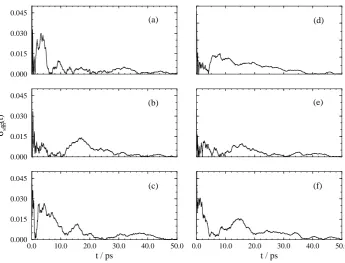
[image:11.595.134.480.81.344.2]rel
Figure 5: Relative errors from transformation 3. For key see Figure 3.
also calculated the difference between the SPC/E and SPC models by a slow growth procedure using a cutoff of 9 ˚A and a simulation time of 70 ps; this determined the stability of SPC/E to be -3.443
±0.003 kJ/mol. In this case the use of the slow growth precedure is seen to produce a result in very close accord with the thermodynamic integration results reported in this study.
The results of this study agree well with those of Hermans et al.,9although as mentioned previously the results of Hermans were not calculated directly but rather are differences between values for the excess free energy of the liquid models. The values of -3.4, 4.2 and -0.8 for transformations 1, 2 and 3 repectively, are in close accord with the values of this study. However, as the values are the difference between the results of two simulations each having an error of at least 0.4 kJ/mol, the results reported in this study have an associated error at least an order of magnitude below these values.
The results of Table 8 indicate an order of stability for the water models at 300 K and 1 atm of SPC/E
0.0 0.2 0.4 0.6 0.8 1.0
λ
−3.60 −3.50 −3.40 −3.30
〈∂
H/
∂λ
〉λ
/
[image:12.595.157.410.171.364.2](kJ/mol)
Figure 6: Results of transformation 1. The dashed line is the result of linear regression.
Transformation ∆G/ (kJ/mol)
Total Constraint Lennard-Jones Coulombic
1 -3.462±0.005 — — -3.462±0.005
2 4.216±0.025 3.585±0.024 -1.017±0.004 1.648±0.005 3 -0.746±0.006 -3.296±0.008 0.937±0.005 1.613±0.003 Cycle 0.008±0.026 0.289±0.025 -0.080±0.006 -0.201±0.008
[image:12.595.80.513.564.651.2]0.0 0.2 0.4 0.6 0.8 1.0 λ 3.0 3.5 4.0 4.5 〈∂ H/ ∂λ 〉λ /(kJ/mol)
0.0 0.2 0.4 0.6 0.8 1.0
3.5 4.0 4.5 5.0 〈∂ H/ ∂λ 〉λ /(kJ/mol)
0.0 0.2 0.4 0.6 0.8 1.0
λ 1.5
1.6 1.7 1.8
0.0 0.2 0.4 0.6 0.8 1.0
[image:13.595.132.478.100.348.2]−1.2 −1.1 −1.0 (a) (b) (c) (d)
Figure 7: Results of transformation 2. The plots are: (a) total derivatives; (b) constraint derivatives; (c) Lennard-Jones derivatives and (d) Coulombic derivatives. The dashed line in each case is the result of linear regression.
0.0 0.2 0.4 0.6 0.8 1.0
λ −3.60 −3.40 −3.20 −3.00 〈∂ H/ ∂λ 〉λ /(kJ/mol)
0.0 0.2 0.4 0.6 0.8 1.0
−1.00 −0.90 −0.80 −0.70 −0.60 −0.50 〈∂ H/ ∂λ 〉λ /(kJ/mol)
0.0 0.2 0.4 0.6 0.8 1.0
λ 1.50 1.55 1.60 1.65 1.70
0.0 0.2 0.4 0.6 0.8 1.0
0.91 0.92 0.93 0.94 0.95 (a) (b) (c) (d)
[image:13.595.118.478.467.719.2]4
Conclusion
We have calculated precise values for the free energy differences between three 3-point models of liquid water. The order of stability if SPC/E >SPC >TIP3P. It is seen that the increased dipole moment of the SPC/E model compared to that of the SPC model lowers the free energy of the former by 3.462±0.005 kJ/mol. The TIP3P model also has an enhanced dipole moment with respect to the SPC model, yet the latter is more stable by 0.746±0.026 kJ/mol, with the effect of constraint and Lennard-Jones terms together being dominant.
The calculations reported here show that small free energy differences can be determined by ther-modynamic integration and molecular dynamics with good precision. This is clearly helped by the fact that the derivative of the Hamiltonian as a function of the coupling paperameter is linear and hence error due to integration can be both reduced and accurately estimated.
The results will have a significance for the qualitative discussion of results obtained with differenct water models. For example, if one is comparing values of hydration free energies calculated in a TIP3P solvent with respect to a SPC/E one, then one must bear in mind that the solvent-solvent free energy may well differ by as much as 4 kJ/mol or more, and hence could significantly affect the comparison.
References
[1] Berendsen, H. J. C., Postma, J. P. M., van Gunsteren, W. F., and Hermans, J. In Intermolecular
Forces, Pullman, B., editor, 331–342. Reidel, Dordrecht (1981).
[2] Berendsen, H. J. C., Grigera, J. R., and Straatsma, T. P. J. Phys. Chem. 91, 6269–6271 (1987).
[3] Jorgensen, W. L., Chandrasekhar, J., Madura, J. D., Impey, R. W., and Klein, M. L. J. Chem.
Phys. 79, 926 (1983).
[4] van Gunsteren, W. F., Billeter, S. R., Eising, A. A., H¨unenberger, P. H., Kr¨uger, P., Mark, A. E., Scott, W. R. P., and Tironi, I. G. Biomolecular Simulation: The GROMOS96 Manual and User
Guide. BIOMOS b.v., Laboratory of Physical Chemistry, ETH Zentrum, Z¨urich, (1996).
[5] Pearlman, D. A., Case, D. A., Caldwell, J. W., Ross, W. S., Cheatham III, T. E., Ferguson, D. M., Seibel, G. L., Singh, U. C., Weiner, P. K., and Kollman, P. A. AMBER 4.1. University of California, San Fransisco, (1995).
[6] Mezei, M. Mol. Phys. 47, 1307–1315 (1982).
[7] Stillinger, F. H. and Rahman, A. J. Chem. Phys. 68, 666 (1978).
[8] Quintana, J. and Haymet, A. D. J. Chem. Phys. Lett. 189, 273–277 (1992).
[9] Hermans, J., Pathiaseril, A., and Anderson, A. J. Am. Chem. Soc. 110, 5982–5986 (1988).
[11] McQuarrie, D. A. Statistical Mechanics. Harper & Row, New York, (1976).
[12] King, P. M. In Computer Simulation of Biomolecular Systems Theoretical and Experimental
Applications, van Gunsteren, W. F., Weiner, P. K., and Wilkinson, A. J., editors, volume 2,
chapter 12, 267–314. ESCOM, Leiden (1993).
[13] van Gunsteren, W. F., Beutler, T. C., Fraternali, F., King, P. M., Mark, A. E., and Smith, P. E. In Computer Simulation of Biomolecular Systems Theoretical and Experimental Applications, van Gunsteren, W. F., Weiner, P. K., and Wilkinson, A. J., editors, volume 2, chapter 13, 315– 348. ESCOM, Leiden (1993).
[14] Ryckaert, J.-P., Ciccotti, G., and Berendsen, H. J. C. Journal of Computational Physics 23, 327–341 (1977).
[15] Berendsen, H. J. C., Postma, J. P. M., van Gunsteren, W. F., DiNola, A., and Haak, J. R. J.
Chem. Phys. 81, 3684–3690 (1984).
[16] Allen, M. P. and Tildesley, M. P. Computer Simulation of Liquids. Oxford University Press, Oxford, (1987).
[17] Beutler, T. C., B´eguelin, D. R., and van Gunsteren, W. F. J. Chem. Phys. 102(9), 3787–3793 (1995).
[18] Ben-Naim, A. Solvation Thermodynamics. Plenum, New York, (1987).
[19] Hodel, A., Simonson, T., Fox, R. O., and Br¨unger, A. J. Phys. Chem. 97(13), 3409–3417 (1993).
[20] Straatsma, T. P., Zacharias, M., and McCammon, J. A. In Computer Simulation of
Biomolec-ular Systems Theoretical and Experimental Applications, van Gunsteren, W. F., Weiner, P. K.,