BIROn - Birkbeck Institutional Research Online
Anastasiadis, A.D. and Magoulas, George D. (2006) Evolving stochastic
learning algorithm based on Tsallis entropic index. The European Physical
Journal B - Condensed Matter and Complex Systems 50 (1-2), pp. 277-283.
ISSN 1434-6028.
Downloaded from:
Usage Guidelines:
Please refer to usage guidelines at or alternatively
Birkbeck ePrints: an open access repository of the
research output of Birkbeck College
http://eprints.bbk.ac.uk
Anastasiadis, Aristoklis D. and Magoulas, George
D. (2006). Evolving stochastic learning algorithm
based on Tsallis entropic index.
The European
Physical Journal B
-
Condensed Matter and
Complex Systems
50
(1-2) 277-283.
This is an author-produced version of a paper published in The European Physical Journal B - Condensed Matter and Complex Systems (ISSN 1434-6028). This version has been peer-reviewed but does not include the final publisher proof corrections, published layout or pagination.
All articles available through Birkbeck ePrints are protected by intellectual property law, including copyright law. Any use made of the contents should comply with the relevant law. Copyright © EDP Sciences, Società Italiana di Fisica, Springer-Verlag 2006.
Citation for this version:
Anastasiadis, Aristoklis D. and Magoulas, George D. (2006). Evolving stochastic learning algorithm based on Tsallis entropic index.London: Birkbeck ePrints. Available at: http://eprints.bbk.ac.uk/archive/00000502
Citation for the publisher’s version:
Anastasiadis, Aristoklis D. and Magoulas, George D. (2006). Evolving
stochastic learning algorithm based on Tsallis entropic index. The European Physical Journal B - Condensed Matter and Complex Systems50 (1-2) 277-283.
http://eprints.bbk.ac.uk
arXiv:cs.NE/0512037 v2 13 Dec 2005
APS/123-QED
Evolving Stochastic Learning Algorithm Based on Tsallis
Entropic Index
Aristoklis D. Anastasiadis∗ and George D. Magoulas†
School of Computer Science and Information Systems, Birkbeck College, University of London,
Malet Street, London WC1E 7HX, United Kingdom.
(Dated: December 13, 2005)
Abstract
In this paper, inspired from our previous algorithm, which was based on the theory of Tsallis
statistical mechanics, we develop a new evolving stochastic learning algorithm for neural networks.
The new algorithm combines deterministic and stochastic search steps by employing a different
adaptive stepsize for each network weight, and applies a form of noise that is characterized by the
nonextensive entropic index q, regulated by a weight decay term. The behavior of the learning
algorithm can be made more stochastic or deterministic depending on the trade off between the
temperature T and the q values. This is achieved by introducing a formula that defines a time–
dependent relationship between these two important learning parameters. Our experimental study
verifies that there are indeed improvements in the convergence speed of this new evolving stochastic
learning algorithm, which makes learning faster than using the original Hybrid Learning Scheme
(HLS). In addition, experiments are conducted to explore the influence of the entropic indexq and
temperatureT on the convergence speed and stability of the proposed method.
∗Electronic address: [email protected]; AD is also affiliated withLondon Knowledge Lab, University of
London, 23-29 Emerald Street, WC1N 3QS, London, United Kingdom
I. INTRODUCTION
Neural networks are widely used in many classification applications. One of the major
key concept in neural networks is the interaction between microscopic and macroscopic
phenomena. The goal of Feedforward Neural Network (FNN) learning is to iteratively adjust
the weights, in order to globally minimize a measure of the difference between the actual
output of the network and the desired output, as specified by a teacher, for all examples (P)
in a training set [1]:
E(w) =
P
X
p=1
nL
X
j=1
yj,pL −tj,p
2 =
P
X
p=1
nL
X
j=1
σL netLj +θ L j
−tj,p
2
. (1)
where, netL
j is for the j-th node in the l-th layer (j = 1, . . . , nL), the sum of its weighted
inputs. θL
j denotes the bias of the j–th node (j = 1, . . . , Nl) at the l–th layer (l = 2, . . . , L),
and wdenotes the weights w in the network. This equation formulates the energy function,
called error function, to be minimized, in which tj,p specifies the desired response at the
j–th output node for the example p and yL
j,p is the output of the j–th node at layer L that
depends on the weights w of the network, and σ is a nonlinear activation function, such
as the well known logistic function σ(x) = (1 +e−x)−1
. The problem of finding the global
minimum of such a complex cost function, which possesses a large number of local minima,
is considered very difficult task [1].
Statistical mechanical methods have been applied successfully to the study of neural
network models of associative memory [2]. These models are biologically plausible and can
be trained very quickly in some cases, compared with the popular neural networks such
as multi–layered perceptron, which have been shown to work satisfactorily. However, this
model of associative memory has still drawbacks as learning gets stuck at local minima.
A variety of global optimization algorithms have also been introduced over the years to
overcome the problem of local minima. One of the most popular methods is the Simulated
annealing [3]. It uses Boltzmann–Gibbs (BG) statistics at two different steps, namely at the
visitation step, which uses a Gaussian distribution, and at theacceptance step, that uses the
Boltzmann factor [4, 5].
Another approach is based on the use of noise models. Attempts to explore the benefits of
introducing noise during learning have been based on the use of Gaussian distributions[4, 6,
7]. One of the most famous neural model operating with noise is the Boltzmann machine, [4,
laws for describing stationary states and basic time–dependent phenomena, where {pi} are
the probabilities of the microscopic configurations, and K > 0. Also, a form of Langevin
noise has been proved quite effective for neural learning, and has motivated the development
of other methods, such as the Simulated Annealing Rprop–SARprop [8].
The next section briefly describes the recently proposed hybrid learning scheme [9], and
then we introduce the proposed evolving stochastic learning algorithm. Next, results of an
empirical evaluation are presented, demonstrating the effectiveness of the new scheme in
locating acceptable solutions. The paper ends with discussion and concluding remarks.
II. THE EVOLVING STOCHASTIC LEARNING ALGORITHM
The recently proposed Hybrid Learning Scheme (HLS) [9] has been built on ideas from
global search methods. It is worth noting that global search algorithms possess strong
con-vergence properties. However, these methods are computationally expensive [8]. To alleviate
this situation hybrid schemes for neural networks learning have been developed in an
at-tempt to achieve improved convergence rates compared to the standard global optimization,
and in some cases even maintain the guarantee of convergence to a global minimizer [6]. HLS
is a hybrid training algorithm that employs a different adaptive stepsize for each weight.
HLS avoids slow convergence in the flat directions and oscillations in the steep directions,
and exploits the parallelism inherent in the evaluation of learning error E(w) and gradient
∇E(w) by the Resilient Back-Propagation (Rprop) algorithm [10]. Inspired by [6, 11], in
the HLS, noise has been introduced in the training procedure according to a nonextensive
schedule [9]. The HLS also applies the sign–based weight adjustment of Rprop [10], on the
perturbed energy function (for a detailed description see [9]).
The new Evolving Stochastic Learning Algorithm (ESLA) introduces noise, as in HLS.
The noise source is characterized by the nonextensive entropic index q. In particular, the
principles of the new method are using the notion of nonextensive entropy, which has been
defined as [12]:
Sq ≡K
1−PW i=1p
q i
q−1 (q ∈R), (2)
where W is the total number of microscopic configurations, whose probabilities are {pi},
and K is a conventional positive constant. When the entropic index q = 1, (2) recovers
to Boltzmann–Gibbs entropy. The entropic index works like a biasing parameter: q < 1
events (values ofp close to 1). The optimization of the entropic form (2) under appropriate
constraints, [12], yields for the canonical ensemble
pi ∝[1−(1−q)βEi]
1
(1−q) ≡e−βEi
q , (3)
whereβis a Lagrange parameter,{Ei}is the energy spectrum, and theq-exponential function
ex
q ≡[1 + (1−q)x]
1 (1−q) =
1
[1−(q−1)x](q−11)
(4)
In this method, like in the HLS, noise is generated according to a schedule:
Q(T, k) =e−T(ln 2)·k
q = [1−(1−q)T(ln 2)·k]
1
1−q, (5)
where T is the temperature; k indicates iterations. Noise is not applied proportionally to
the size of each weight; instead a form of weight decay is used, which is considered beneficial
for achieving a robust neural network that generalizes well. Thus, noise is introduced by
formulating the perturbed energy function:
˜
E(wk) =E(wk) +µ·
n X
i=1
(wk i)
2
[1 + (wk i)
2
] ·Q(T, k), (6)
where E(w) is the error function, P
iw2i/(1 +w2i) is the weight decay bias term which can
decay small weights more rapidly than large weights, and µ is a parameter that regulates
the influence of the combined weight decay/noise effect. The energy landscape is modified
during training so the search method is allowed to explore regions of the energy surface that
were previously unavailable. Minimization of (6) requires calculating the gradient of the
energy with respect to each weight
˜
gi(wk) =gi(wk) +µ´·
wk i
[1 + (wk i)
2
]2 ·Q(T, k), (7)
where gi(wk) is the gradient of the energy E(wk), with respect to each weight, and µ´> 0
(in our experiments a fixed value of µ´= 0.01 was used). The proposed evolving stochastic
hybrid scheme applies a sign–based weight adjustment, similar to HLS [9], on the perturbed
energy function (6) using the gradient term of Equation (7). Also the learning rates are
adapted by Rprop learning procedure [10].
In our approach the weight adjustment is given by the following equation:
wk+1=wk−τkdiag{ηk
1, . . . , ηik, . . . , η k
where sign(˜gi(wk)) denotes the column vector of the signs of the components of ˜g(wk) =
˜
g1(wk),˜g2(wk), . . . ,˜gn(wk)
, τk >0, ηk
m (m= 1,2, . . . , i−1, i+ 1, . . . , n) are small positive
real numbers generated by Rprop’s learning rates schedule.
Moreover, an additional condition, like in the HLS, is introduced in order to avoid using
relatively small weight adjustments
if ηik−1 < ρ·Q2(T, k)
then
ηik =max
ηik−1η
−
+ 2cρ·Q2(T, k),∆min
, (9)
where 0< ρ < 1 and c∈(0,1) is a random number.
Lastly, inspired from previous work, [11], we apply a cooling procedure. This defines the
relationship betweenT andqvalues. The application of cooling helps to regulate the training
algorithm, making it more deterministic. This new Evolving Stochastic Learning Algorithm -ESLA behaves in a more stochastic way, during the initial stages, and then becomes more
deterministic as the number of iterations increases. Thus, when we are close to the minimizer,
the algorithm hopefully will avoid oscillations and converge faster. The cooling procedure
is described by the next equation:
T =T0·[
2q−1−1
(1 +k)q−1−1], q >1 (10)
where T0 is the initial temperature, T is the current temperature, k is the number of
itera-tions, and q is the Tsallis entropic index.
The challenge is to cool the temperature the quickest we can, but still having the ability
to converge to global minimum with high probability. The standard simulated annealing
(SA) is one method to achieve this goal. However, the cooling procedure is computationally
expensive. An efficient alternative cooling method is the fast simulated annealing (FSA) [13].
The temperature is now allowed to decrease like the inverse of time, which makes the entire
cooling procedure quite more efficient. Simulated annealing (GSA) [11] is a generalization
of the previous methods, which performs better than previous annealing algorithms for
many problems and applications. In neural networks applications we are mainly interested
in accelerating the learning speed with no affect in generalization. The cooling procedure
based on GSA satisfies these two targets and contributes positively to the performance of
the ESLA. This cooling procedure makes the temperature to decrease as a power-law of
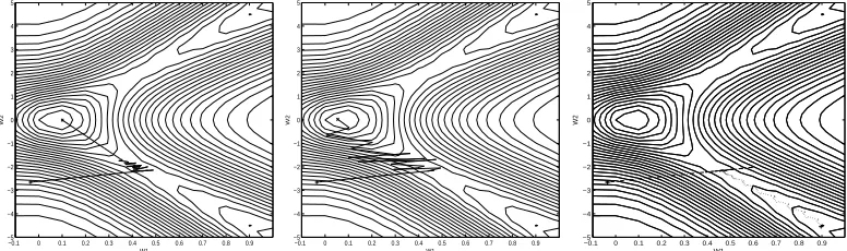
Below, a simple problem is used to visualize the behavior of the ESLA and compare it
with the HLS, and the Rprop algorithm. The energy landscape of Figure 1 has a global
minimum and two local minima. Figure 1 shows that under the same initial conditions,
both of the ESLA and the HLS escape the saddle point and the valley that leads to a local
minimum, while the ESLA converges faster than HLS with fewer oscillations(Figure 1, left),
and the Rprop algorithm converges to the local minimizer (Figure 1, right).
−0.1 0 0.1 0.2 0.3 0.4 0.5 0.6 0.7 0.8 0.9 −5 −4 −3 −2 −1 0 1 2 3 4 5 W1 W2
−0.1 0 0.1 0.2 0.3 0.4 0.5 0.6 0.7 0.8 0.9 −5 −4 −3 −2 −1 0 1 2 3 4 5 W1 W2
[image:8.612.110.498.201.316.2]−0.1 0 0.1 0.2 0.3 0.4 0.5 0.6 0.7 0.8 0.9 −5 −4 −3 −2 −1 0 1 2 3 4 5 W1 W2
FIG. 1: Weights trajectories of the Evolving Stochastic Learning Algorithm–ESLA (left), the
Hybrid Learning Scheme–HLS (center), and the Rprop (right).
III. EXPERIMENTAL STUDY
We have evaluated the performance of the ESLA and compared it with the Rprop, and
the HLS algorithms. The statistical significance of the results has been analyzed using the
Wilcoxon test [14]. This is a nonparametric method that is considered an alternative to the
paired t–test. All statements in the tables reported below, refer to a significance level of
0.05. Statistically significant cases are marked with (+), while (−) shows the cases that don’t
satisfy the significance level. Moreover, the following terms are used: Epochsis the number
of iterations to converge to the error target;Convergencedenotes the success of convergence
to the error target within 2000 iterations; Generalization is the percentage of correctly
classified test examples. Finally, for all the the problems we have set the initial temperature
toT = 2 for training using the ESLA. By keeping constant the initial temperature we found
the optimal value for the Tsallis entropic indexq. The parameters of the HLS were set to the
same values as in the ESLA for all experiments in an attempt to test the robustness of the
method in different types of problems: the temperature is equal to the initial temperature
T = 2, and the q is set in different values depending on the problem, (i.e. in cancer T = 2
trials. These 300 random weight initializations have been the same for the three learning
algorithms.
A. Benchmarks from the UCI Repository
The data sets for the cancer1, diabetes1, thyroid1 problems were used as supplied on
the PROBEN1 website. PROBEN1 provides explicit instructions for creating training and
testing sets and choosing network architectures for many problems [15]. The partitioning
is 50% of the full data is used as training set, then the next 25% of the dataset is used as
validation set, and the remaining 25% as testing set. The diabetes1 benchmark is a real-world classification task which concerns deciding when a Pima Indian individual is diabetes
positive or not [15, 16]. The Proben1 collection suggests a 8–2–2–2 FNN. The termination
criterion is E ≤ 0.14 within 2000 iterations. In order to find the best value for the initial
temperature and the tsallis entropic index q, we performed 30 different runs. Figure 2 shows the ESLA’s performance for an initial temperature T = 2 and different q values.
Judging from the Figure 2 the best value for q = 1.6, and T = 2. Table I shows that
1.1 1.2 1.3 1.4 1.5 1.6 1.7 1.8 1.9 0 500 1000 1500 2000 2500 Diabetes q values Epochs
1.1 1.2 1.3 1.4 1.5 1.6 1.7 1.8 1.9 74.6 74.8 75 75.2 75.4 75.6 75.8 76 76.2 q values Generalization Diabetes
1.1 1.2 1.3 1.4 1.5 1.6 1.7 1.8 1.9 2 300 400 500 600 700 800 900 1000 1100 Cancer q values Epochs
1.1 1.2 1.3 1.4 1.5 1.6 1.7 1.8 1.9 2 97.25 97.3 97.35 97.4 97.45 97.5 97.55 97.6 97.65 97.7 Cancer q values Generalization
FIG. 2: Optimal q based on Epochs, and Generalization for the diabetes (two left plots), and
cancer problems.
the Rprop algorithm converges many times in local minima. The new stochastic learning
algorithm overcomes this problem in most of the cases. The cooling procedure seems to
have a positive impact on the learning speed of the algorithm. The second benchmark is
the breast cancer diagnosis problem which classifies a tumor as benign or malignant based
on 9 features [15, 16]. We have used an FNN with 9–4–2–2 nodes, as suggested in [15], and
a termination criterion of E ≤0.02. Figure 2 shows the best values of these two important
training parameters. As we can observe from this figure, a value of the q = 1.7 gives the best results in terms of both learning speed and generalization. The comparative results are
TABLE I: Comparison of algorithms performance in the Diabetes and Cancer problems for the
converged runs
Diabetes Cancer
Algorithm Epochs Generalization Convergence Epochs Generalization Convergence
Rprop 700 (+) 75.2 (%) (+) 86 (%) (+) 287 (+) 97.2(%) (−) 94(%) (+) HLS 570 (+) 75.8 (%) (+) 94 (%) (−) 230 (+) 97.4(%) (−) 96(%) (+)
ESLA 480 76.2 (%) 95 (%) 195 97.4(%) 99(%)
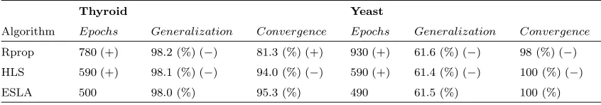
The third benchmark problem is thethyroid1, which is not a permutation of the original data, but retains the original order instead [15, 16]. The data set consists of 3600 patterns.
The termination criterion is E ≤ 0.0036. The Tsallis entropic index q in this problem is
again q= 1.7. The experimental results that we obtained are presented in Table II.
1.1 1.2 1.3 1.4 1.5 1.6 1.7 1.8 1.9 600 800 1000 1200 1400 1600 1800 2000 2200 q values Epochs Thyroid
1.1 1.2 1.3 1.4 1.5 1.6 1.7 1.8 1.9 2 75 80 85 90 95 100 q values Generalization Thyroid
1.1 1.2 1.3 1.4 1.5 1.6 1.7 1.8 1.9 500 1000 1500 2000 2500 3000 3500 Yeast q values Epochs
[image:10.612.77.538.261.379.2]1.1 1.2 1.3 1.4 1.5 1.6 1.7 1.8 1.9 63.35 63.4 63.45 63.5 63.55 63.6 63.65 Yeast q values Training Generalization
FIG. 3: Optimalqbased on Epochs, and Generalization for the thyroid (two left plots), and Yeast
problems.
TABLE II: Comparison of algorithms performance in the Thyroid and Yeast problems for the
converged runs
Thyroid Yeast
Algorithm Epochs Generalization Convergence Epochs Generalization Convergence
Rprop 780 (+) 98.2 (%) (−) 81.3 (%) (+) 930 (+) 61.6 (%) (−) 98 (%) (−) HLS 590 (+) 98.1 (%) (−) 94.0 (%) (−) 590 (+) 61.4 (%) (−) 100 (%) (−) ESLA 500 98.0 (%) 95.3 (%) 490 61.5 (%) 100 (%)
B. Prediction of Localisation sites of the Yeast Proteins
The study of protein localization is considered very useful in the post-genomics and
proteomics era, as it provides information about each protein that is complementary to the
protein sequence and structure data [17]. One of the most thoroughly studied single–cell
[image:10.612.93.516.518.592.2]rate and very simple nutritional requirements [18]. The Yeast dataset is 1484 proteins
labeled according to 10 sites [19]. Yeast proteins are organized as in [16]. The most suitable
architecture for this problem, as suggested by [20], is an 8-16-10 FNN architecture. A
termination criterion of E ≤ 0.05 within 2000 iterations (Epochs) is used. The evaluation
method that we have employed to estimate the accuracy of the methods was a 10-fold cross
validation following the guidelines of [19, 20]. The proportion of the number of the patterns
for all the classes is equal in each partition, as this procedure provides more accurate results
than a plain cross validation does [21]. Figure 3 gives an overview of the experiments
conducted in order to choose the best value of q for this problem. A value of q = 1.6 was
applied as this gave the best results in terms of learning speed and generalization. Table II
shows the experimental results for this difficult problem.
C. Boolean function approximation problems
Another set of experiments has been conducted to empirically evaluate the performance
of the new method in a well–studied class of boolean function approximation problems that
exhibit strong local minima [22]. This class includes the XOR problem, and the parity–
3 problem, which is considered as classic benchmarks [8, 9]. The adopted architectures
for the XOR problem is a 2–2–1, and the error target was set to E ≤ 10−5. A 3–3–1
architecture was used for the parity–3 problem. The error target for parity-3 problem was
set to E ≤5×10⁻⁵. The activation function for this problem is the tansig function. These
target values are considered low enough to guarantee convergence to a “global” solution. By applying the same procedure as before, the best q entropic index value for the XOR
problem is q = 2.1, and for the parity 3 problem is q= 1.1 with initial temperature T = 2.
Table III shows that the ESLA outperforms in convergence speed. The HLS achieves the
best Convergence success on XOR problem. However, the ESLA has better convergence
[image:11.612.90.519.651.723.2]performance compared to Rprop.
TABLE III: Comparison of algorithms performance in the XOR and Parity 3 problems for the
converged runs
XOR Parity3
Algorithm Epochs Generalization Convergence Epochs Generalization Convergence
Rprop 120 (+) 100 (%) (−) 59 (%) (+) 877 (+) 100 (%) (−) 74 (%) (+) HLS 80 (+) 100 (%) (−) 68 (%) (−) 430 (+) 100 (%) (−) 78 (%) (+)
IV. DISCUSSION AND CONCLUDING REMARKS
A recently introduced training algorithm, the hybrid learning scheme-HLS achieves
gen-erally very good and reliable performance, and improved learning speed compared to the
Rprop algorithm. In this paper, we proposed a new evolving stochastic learning scheme,
which constitutes an efficient improvement of the HLS algorithm that is built on a
theoreti-cal basis. The ESLA combines deterministic and stochastic search by employing a different
adaptive stepsize for each weight, and a form of noise that is characterized by the
nonex-tensive entropic index q. An adaptive formula that introduces a relationship between the
T and q was applied. Our experimental study showed that there is a range of q values
(1.1< q <2.3) that gives good performance for the new learning scheme.
In previous tables the results are based only on the converged runs. Therefore, we don’t
have the actual performance description of the tested algorithms (i.e. in thyroid problem the Rprop algorithm achieves the best mean generalization success. However, its
conver-gence success is the worst within the tested algorithms. Therefore, the converconver-gence results
present the Rprop’s generalization for the 0.813·300 = 244 runs out of 300, while the mean
generalization success of ESLA is based on 0.953· 300 = 286 runs out of 300). In this
case it is better to have results for more runs (i.e. patients) although the generalization success is slightly worse. In order to have better view of the overall performance of the
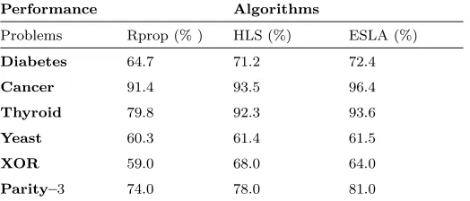
tested algorithms, we introduce the parameter Performance, which is defined as follows:
Performance = (Convergence)×100(Generalisation). Thus, Table IV gives a summary of our results
[image:12.612.176.438.542.654.2]from this perspective for all the tested algorithms.
TABLE IV: Summary of the results in terms of the algorithms’ Performance
Performance Algorithms
Problems Rprop (% ) HLS (%) ESLA (%)
Diabetes 64.7 71.2 72.4
Cancer 91.4 93.5 96.4
Thyroid 79.8 92.3 93.6
Yeast 60.3 61.4 61.5
XOR 59.0 68.0 64.0
Parity–3 74.0 78.0 81.0
Further testing is of course necessary to fully explore the advantages and identify possible
limitations of this cooling evolving scheme. Moreover, exhaustive testing of the new method
in a restarting mode. Finally, we are going to explore further the properties of Tsallis entropy
into Optimization methods in Artificial Intelligence applications.
V. ACKNOWLEDGEMENTS
Aristoklis Anastasiadis would like to thank Dr. G. Kaniadakis and would also like to
address special thanks to Prof. Constantino Tsallis for very helpful discussions related to
this work, during his stay as research visitor at the Santa Fe Institute.
[1] S. Haykin, Neural Networks: A Comprehensive Foundation, Macmillan College Publishing
Company, 1994.
[2] G. Gyorgyi, Techniques of replica symmetry breaking and the storage problem of a
McCulloch-Pitts neuron”, Physics Reports, Vol. 342, issue 4-5, pages 263-392, 2001.
[3] S. Kirkpatrick, C.D. Gelatt Jr., and M.P. Vecchi, Optimization by simulated annealing.
Sci-ence, 220, 671–680, 1983.
[4] D. Ackley. G. Hinton and T. Sejnowski, A learning algorithm for Boltzmann machines.Cogn.
Sci., 9, 147–169, 1985.
[5] E. H. L. Arts and J. Korst,Simulated Annealing and Boltzmann Machines. New York: Wiley,
1989.
[6] R. M. Burton and G. J. Mpitsos, Event dependent control of noise enhances learning in neural
networks. Neural Networks, 5, 627-637, 1992.
[7] T. R¨ognvaldsson, On Langevin updating in multilayer perceptrons. Neural Computation, 6,
916–926, 1994.
[8] N. K. Treadgold and T. D. Gedeon, Simulated Annealing and Weight Decay in Adaptive
Learning: The SARPROP Algorithm. IEEE Tr. Neural Networks, 9, 4, 662–668, 1998. [9] A.D. Anastasiadis, G.D. Magoulas, “Nonextensive statistical mechanics for hybrid learning of
neural networks’, Physica A, vol.344, pp. 372-382, 2004.
[10] M. Riedmiller and H. Braun, A direct adaptive method for faster backpropagation learning:
The Rprop algorithm. Proc. Int. Conf. Neur. Net., San Francisco, CA, 586-591, 1993.
[11] C. Tsallis and D. A. Stariolo, Generalized Simulated Annealing. Physica A, 233, 395–406,
1996.
[12] C.Tsallis, Possible Generalization of Boltzmann-Gibbs Statistics. J. Stat. Phys., 52, 479–487,
1988.
[13] H. Szu, Nonconvex optimization by fast simulated annealing.Proceedings of IEEE, 75, 1538–
[14] G. Snedecor and W. Cochran, Statistical Methods, Iowa State University Press, 8th edition,
1989.
[15] L. Prechelt, PROBEN1–A set of benchmarks and benchmarking rules for neural network
training algorithms, Technical report 21/94, Fakultt fr Informatik, Universitt Karlsruhe, 1994. [16] P.M. Murphy and D.W. Aha, UCI Repository of machine learning databases,
http://www.ics.uci.edu∼mlearn/MLRepository.html., 1994.
[17] M.V. Boland and R.F. Murphy, After sequencing: quantitative analysis of protein localization,
IEEE Engineering in Medicine and Biology, Sept/Oct., 115-119, 1999.
[18] H. Lodish, A. Berk, S.L. Zipursky, P. Matsudaira, D. Baltimore, and J. James Darnell,
Molec-ular Cell Biology, Freeman, 5th edn, 2003.
[19] P. Horton, and K. Nakai, Better Prediction of Protein Cellular Localization Sites with the k
Nearest Neighbors Classifier. Proc. ofIntelligent Systems in Molecular Biology, 368-383, 1997. [20] A.D. Anastasiadis, G.D. Magoulas and X. Liu, Classification of protein localisation patterns
via supervised neural network learning, Proc. of the Fifth Symposium on Intelligent Data
Analysis,Lecture Notes in Computer Science, vol. 2810, Springer-Verlag, 430–439, 2003.
[21] R. Kohavi, A study of cross-validation and bootstrap for accuracy estimation and model
selection, International Joint Conference on Artificial Intelligence, pp. 223-228, 1995.
[22] E.K. Blum, Approximation of Boolean functions by sigmoidal networks: Part I: XOR and