Representation and reasoning: a causal model approach

(1)

Representation and Reasoning

A Causal Model Approach

By Milena Nikolic

Cognitive, Perceptual and Brain Sciences Research Department University College London

Thesis submitted for the degree of Doctor in Philosophy (PhD)

(2)

Thesis Declaration

I declare that this thesis was composed by myself and that the work contained herein is my own except where explicitly stated otherwise in the text. This work has not been submitted for any other degree or professional qualification.

Signature:

(3)

Abstract

How do we represent our world and how do we use these representations to reason about it? The three studies reported in this thesis explored different aspects of the answer to this question. Even though these investigations offered diverse angles, they all originated from the same psychological theory of representation and reasoning. This is the idea that people represent the world and reason about it by constructing dynamic qualitative causal networks. The first study investigated how mock jurors represent criminal evidence and reason with such representations. The second study examined how people represent the causes of a complex environmental problem and how their individual representations are directly linked to how they reason about the issue. The third and final study inspected how people represent causal loops and reason in accordance with these cyclical representations. These studies suggest that people do represent the world by arranging evidence, causes, or pieces of information into a causal network. In addition, the studies support the idea that these networks are of a qualitative nature. All three studies also indicated that people update their representations in accordance to a dynamic world. The studies specifically explored how reasoning, and therefore judgment is linked to these representations. The thesis discusses the theoretical implications of these and other findings for the causal model framework as well as for cognitive science more generally. Related practical implications include the importance of understanding naïve causal models for applied fields such as legal decision-making and environmental psychology.

(4)

(5)

Acknowledgements

Foremost, I would like to express my deepest gratitude to my supervisor Dave Lagnado. I consider myself exceptionally lucky to have had the privilege of being supervised by somebody who has been the greatest inspiration both as an academic and as a person. I thank him for his infinite guidance, help and understanding. I could not have imagined having a better supervisor and mentor for my Ph.D. study.

I would also like to thank all the members of my lab for always being there to give me valuable feedback. In particular, I would like to thank Adam Harris, Tobias Gerstenberg, Christos Bechlivanidis , Chris Olivola, Anne Hsu and Cristina Miclea for all their time and help through my research. Special thanks to Professor David Green, for his time consulting on some of the integral ideas in this thesis.

Finally, I would like to thank all of my amazing family. Thanks to my parents, Mamma and Pappi, for always being there for me in every possible way. Thanks to my sisters, Vali and Irene, for all their understanding throughout these last four years. Thanks to my grandparents, Dodo and Nonna. Thanks to my little friend Zen.

(6)

4.1 Introduction ……….102 4.2 Experiment 1 ………...113 4.3 Method ………...117 4.4 Results ……….122 4.5 Discussion………133 4. 6 Experiment 2 ………..………135 4.7 Method ………..………..137 4.8 Results ……….140 4.9 Discussion ………...145 4.10 Experiment 3……..………147 4.11 Method ………..149 4.12 Results ………...154 4.13 Discussion ……….175 4.14 Experiment 4………..179 4.15 Method ………..179 4.16 Results ………...181 4.17 Discussion ……….193 4.18 General Discussion……….196 5 Discussion 211 5.1 Theoretical implications………...211

(8)

5.2 Practical implications………...214

5.3 Experimental considerations………216

5.4 Future directions………...217

6 References 219

(9)

Chapter 1: Introduction

The introduction starts by presenting the question that has driven the research reported in this thesis. The what, the why and the how are discussed to provide a brief idea of the rationale behind the question as well as the chosen approach. This is followed by an overview of the general background that forms the basis of the studies discussed in the ensuing three chapters. Finally, a brief outline describes the research question of each study.

1.1 The question What?

The central premise of cognitive science is that thinking can best be understood in terms of representational structures in the mind and computational procedures that operate on those structures. This hypothesis can be framed into one question: “How do we represent our world and how do we use these representations to reason about it?” In a sense, this question encompasses two enquiries within one: the question of representation and the question of reasoning. These stand by themselves, but they are intrinsically interrelated in every way. Arguably, there cannot be one without the other. This thesis focuses exactly on investigating the nature of this interrelation and how it may shape judgment and decision-making in different aspects of everyday life.

Why?

The dominant tenet behind this question is that the quest of answering it yields important theoretical as well as practical implications. From a theoretical standpoint,

(10)

the question of representation and reasoning lies at the very core of most theories of how the mind works. This means that attempting to further comprehend how people understand the world and make decisions based on this understanding, will inform current theoretical accounts. From a practical perspective, there is much to be gained from adopting an applied approach. Understanding the driving forces that underlie people’s decisions and actions can potentially help unlock solutions to many of today’s complex problems (White, 2000).

How?

The question of how people represent the world and reason with these representations is complicated by the fact that the world is always changing. The very course of Nature is about change on every level. Everything with a physical realization is transient: the way in which seeds sprout, species evolve and oceans warm are just a few simple examples. Therefore reasoning and representation cannot possibly be based on these unstable states. Rather, it must be based on the idea that events do indeed change but the forces of change do not – they remain invariant across spatial and temporal contexts.

These forces of change are simply mechanisms of cause and effect. The temperature of the ocean is always changing - it is unstable. However, the causal relations that govern the mechanisms by which it warms up are invariant: more carbon dioxide in the atmosphere will always cause the ocean to warm up. This concept is embodied in the principle of causal invariance (Sloman 2009; Woodward, 2000). Accordingly, the causal relations that govern mechanisms of change form a reliable basis for general knowledge. After all, science is concerned precisely with discovering and representing causal structure - be it how force changes acceleration or

(11)

how overfishing changes ecosystems. The point is that the casual principles that govern mechanisms are useful because they apply across time and across a large number of objects – in other words, they allow generalization of empirical knowledge. Hence, it follows then that the logic of causality is people’s guide to prediction, explanation and action. This logic is the tenet of the causal model framework (Pearl, 2000; Spirites, Glymour and Scheines, 1993) and will be used to approach the question of reasoning and representation.

1.2 Representation and reasoning

There have been substantial advances in normative models of both representation and reasoning over the past decade, and a variety of network models have been developed. Network models are simply graphical representations of causal relations (links) between events or causes (nodes). These include Wigmore charts (Wigmore, 1913), cognitive maps (Axelrod, 1976), and Bayesian networks (Pearl, 1998). Given that the central question concerns reasoning as well as representation, the only relevant network model is Bayesian networks. This is because a significant feature of Bayesian networks is that once the representation is constructed, it can be used for inference. This sets it apart from most other forms of networks (e.g. Wigmore charts and Cognitive maps), which serve mainly as descriptive tools. Indeed representation is intertwined with inference in a Bayesian network (Lagnado, 2011). Bayesian networks are directed acyclic graphs in which the nodes represent the variables relevant to the situation (e.g., the presence of an alibi, the number of fish in the sea, the occurrence of an event) and the links represent causal relations among these variables. The strength of a causal relation is defined by conditional probabilities that are related to each collection of parents–child nodes in the network.

(12)

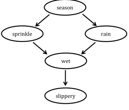
Figure 1 shows an example of a Bayesian network based on a classic example adapted from Pearl (2000).

The network in the figure describes the causal relationships among the following variables; season of the year (season), whether rain falls (rain) during the season, whether the sprinkler is on (sprinkler) during that season, whether the pavement would get wet (wet), and whether the pavement would be slippery (slippery). In this example, the lack of a direct link between ‘season’ and ‘slippery’ captures the idea that changes in season affect the slipperiness of the pavement by other intermediate factors (e.g., how wet the pavement is).

Figure 1

A Bayesian network representing causal influences among five variables.

Perhaps the most important thing to note in this example is that a Bayesian network models the environment as opposed to modeling a reasoning process. This is not the case in many other knowledge representation schemes like logic, rule-based systems, and neural networks. The fact that a Bayesian network simulates the causal

sprinkle r slippery season rain wet

(13)

mechanisms in the environment means that it allows people to represent the world as it is. This implies that they can then answer a range of questions based on this representation. Such questions might include abductive questions, such as “What is the most plausible explanation for the pavement being wet?” and control questions, such as “What will happen if we switch off the sprinkler?” It is clear that the answers to these questions are based on the causal knowledge that can effectively be represented and processed in Bayesian networks.

Bayesian networks have well-established foundations in probability theory, and are currently applied in many practical contexts (e.g. medical diagnosis; Heckerman, 1991). Evidently, this formal approach is just prescriptive in the sense that it does not necessarily reflect the psychological reality of representation and reasoning. People do not always represent probability distributions accurately and do not always make sound probability judgments as set by causal model theory (Gilovich, Griffin and Kahneman, 2002; Kahneman, Slovic and Tversky, 1982). The question of how people really represent and reason necessitates a descriptive approach instead – an approach based on the causal model framework as a psychological theory (Sloman, 2005). This is not to say that a descriptive approach completely discards the prescriptive causal model theory. On the contrary, it can very much be based on some of the same core ideas. What follows is a brief description of some (by no means all of them) of these core ideas. These concepts shape the psychological theory of representation and reasoning that will guide the investigation of the central question put forward by the current thesis.

Causal networks

(14)

is that people’s representations are in the form of a network. This is the intuitive notion that individual cause-effect relations are not isolated from each other but tend to be understood in an organized representation of chains and networks of causal relations (White, 2008). This network arrangement lets people deal with complex multivariate causal reasoning: reasoning based on numerous interrelated pieces of information. This is because the whole is more than the sum of its parts. In other words, the structure of a causal belief system (a set of interrelated causal relations) is more informative than the isolated individual beliefs (Waldman & Hagmayer, 2005).

For example, if a tree was to be reduced to its individual parts (leaves, branches, trunk, bark, roots, fruit, and so on) it would not be possible to represent the whole tree’s significance, such as the role the tree plays as habitat for birds, insects, parasitic vines, and other organisms. Similarly, chemically analyzing of the tree’s chloroplasts, diagramming its branch structure, and evaluating its fruit’s nutritional content, would not lead to understanding the tree as habitat, as part of the forest landscape, or as a reservoir for carbon storage.

Hence, the idea is that a cause, or variable within the network, can only be evaluated meaningfully with respect to its relation to other items represented within the network. This is not to say that people do not isolate small fragments of the network they represent - indeed this is what makes the whole network representation tractable for the human mind (Lagnado, 2011).

Qualitative relations

The second idea that provides the key to making causal networks tractable for everyday representation and reasoning is that people represent the qualitative structure of causal systems without actively representing all the quantitative details

(15)

(Wellman & Henrion, 1993). For example, a link from A to B tells us that certain values of A will change the probability of certain values of B, without needing to specify exactly how much.

Indeed, even the network structure underpinning a Bayesian Network is purely qualitative in the sense that it represents the presence or absence of a dependency between a set of variables. Even though the standard Bayesian Network framework requires a precise set of conditional probabilities, many of the important characteristics of the network are retained without a full and exact set of probabilities (Biedermann and Taroni, 2006; Wellman and Henrion, 1993). This means that even if people are unable to perform exact Bayesian computations over this network, they can still draw approximate inferences (perhaps using heuristic methods). There is growing empirical evidence that people reason in accordance with the qualitative prescripts of causal Bayesian Networks (Krynski and Tenenbaum, 2007; Sloman and Lagnado, 2005).

This idea is particularly significant in domains where no precise figures are available or where much of the information does not admit of quantification (there might be large numbers of interacting variables so that exact inference is intractable). For example, as Lagnado points out (2011) it might not be possible to quantify the exact probative force of a witness testimony that places the defendant at the crime scene; but most people would agree that it raises the probability of guilt, however slightly. Moreover, people will often be able to make comparative probability judgments; for instance, judging that a certain piece of forensic evidence raises the probability of guilt more that the testimony of a partial witness.

The idea that people utilize qualitative networks is not new. There are several psychology studies that speak in favour of qualitative approaches. First,

(16)

psychophysical studies show that for a range of sensory phenomena people are poor at making absolute judgements, and instead make ordinal comparisons (e.g. Stewart, Brown and Chater, 2005). Second, analyses of a wide range of predictive tasks (e.g. clinical and medical diagnosis) suggest that statistical models that use unit weights often outperform more complex models (Dawes, 1979). The key requirement for these simpler models is that the sign of each variable in the model is correct, while the exact weights placed on these variables is not significant. The proposed qualitative networks however, go beyond simple linear models, but share the intuition that precision in the weights is not a necessary condition for successful inference.

Dynamic models

The third idea is based on the appreciation that people’ representations must adapt to a changing environment (Osman, 2010). These changes in the environment might involve new information, new hypotheses and new goals (Lagnado, 2011). Most events in everyday life are not detected based on a particular point in time, but they can be described through multiple states of observation that yield a judgment of one complete final event. This implies that many learning experiences involve repeatedly learning about one variable over time (Rottman & Keil, 2012). For example, one might develop beliefs about the causal relationships between fatigue, insomnia, and stress, by observing a person who experiences these conditions wax and wane over time. This temporal dependency of the states between variables is what constitutes a dynamic model.

Indeed, Bayesian Networks can been adapted to model scenarios in which the states of variables are temporally dependent. In these Bayesian Dynamic Networks (DBNs), at each time period the state of a variable is determined both by the causal

(17)

relationships within that time period and also by prior states. An example of a DBN can be seen in Figure 2. Figure 2 shows the relationship between stress, insomnia and fatigue modeled as a causal chain whereby stress affects insomnia, which in turn affects fatigue.

Figure 2.

An example of a dynamic causal model.

According to DBNs, the probabilities associated with each node are updated at each time period. This updating process involves intricate computations that can be executed by computational algorithms, sometimes using only approximate inference due to the computational complexity (e.g., Friedman, Murphy and Russell, 1998). As outlined above, people engage in a form of dynamic updating all the time. Naturally, the way in which they update, however, differs from the strictly Bayesian updating process in which a complete set of hypotheses are continually updated – that would be too demanding on a computational level. Rather, it has been proposed that people introduce and eliminate hypotheses in a more all-or-nothing manner (Lagnado, 2011)

Time Stress Insomnia Fatigue

t0 t1 t… tn S I F S I F S I F S I F

(18)

– which makes inference considerably easier.

This concept fits well with the idea that people’s representations are in the form of a network. This structure allows people to update the representation by recruiting only the relevant fragments of the network – the ones affected by the new information. Similarly, the qualitative nature of the representation means people can easily and readily update their representation without having to carry out numerous probability estimations and computations.

1.3 Outline

The current thesis investigates the answer to the question of reasoning and representation through three related yet distinct studies. All of them seek to explore the connection between representation and reasoning but in different forms.

Before outlining these three studies that form the basis of each of the following chapters, it is worth pointing out two key features they all have in common. The first of these is that they are all based on lay people. This is a crucial point because lay people have a way of representing and reasoning that differs from those of experts (Hoffman, 1996). This is true for most fields - the way a patient represents the causes of heart disease will undoubtedly differ from that of the doctor (Cuthbert, Dubolay, Teather et al., 1999). Similarly, even if lay people and experts were to have the same representations, the inferences drawn from them are bound to differ. Nevertheless, there is much to be learnt from lay people’s representations and reasoning patterns – especially because they form the basis of general decision-making and therefore signify the power of the masses.

This leads to the second feature accompanying these studies: they are all carried out with practical applications in mind. This means that the investigations are

(19)

based on how people represent real world problems and how they might reason about them in an applied context. The applied approach starts off with Study 1, which is based on legal inference with a focus on juror decision-making. What makes the legal domain an appealing field of study is that many of its staple characteristics are also at the core of other significant applied domains. Evidence presented at trials tends to be contradictory, incomplete, biased and available in multiple formats that make them hard to compare and integrate. In addition the verdict needs to be reached under time constraints and limited cognitive resources. It is easy to see how these features are not exclusive to juror decision-making. These attributes are also the ones governing environmental problems, particularly from a consumer’s point of view. The everyday consumer is constantly being fed contrasting evidence about climate change and anthropogenic effects of human behaviour. The information comes in many forms, from news reports, to word-of-mouth. Some of it is in the format of a statistic whilst other is simply a general opinion. Yet consumers have to make decisions that concern the environment everyday, every time they choose one product over another or chose to how to get to work. That is why the second study extends the exploration of representation and reasoning to the applied domain of environmental problems, dealing with one of the most complex contemporary issues of all: overfishing. The third study takes the investigation of the representation and reasoning to simpler domains including sleeping patterns and simple predator-prey relationships. This move to more familiar subjects was necessary to be able to study reasoning based on the more complex representations (causal loops) which drive the final study.

(20)

Study 1: Reasoning with causal evidence: understanding legal inferences.

The first study investigated how mock jurors represent criminal evidence and reason with causal network representations. Specifically, it explored: i) how jurors represent evidence (with a focus on how they update their representations in the face of new evidence); ii) the extent to which they arrange evidence in a causal network structure; and iii) jurors’ ability to make causal inferences in line with their representations.

Study 2: Reasoning with causal networks: understanding environmental problems.

The second study examined how people represent the causes of a complex environmental problem (overfishing) and how their individual representations are directly linked to how they reason about the issue. In particular, it studied: i) whether people construct two-way causal relations (causal loops) within their representations; ii) the relation between the representations and counterfactual judgments; and iii) which features of their representations (e.g. causal strength of relations versus sheer number of causal relations) is most significant in predicting judgments.

Study 3: Reasoning with causal loops: understanding everything.

The third and final study inspected how people represent causal loops and reason in accordance to these cyclical representations. These are a form of simple qualitative dynamic networks. Specifically, the study employed different applied scenarios to survey the extent to which people can make proper causal inferences given the loops portrayed by these situations.

(21)

Chapter 2: Reasoning with causal evidence: understanding

legal inferences

2.1 Introduction

The jury is the only decision-making body in the criminal justice system composed of laypersons and jury verdicts directly affect the implementation of justice in the USA, UK and elsewhere. This means that the lives of hundreds of thousands of individuals around the world every year depend on the fairness of jury decision-making. Researching the psychological processes underlying juror decision making, and the way these relate to formal methods of evidence evaluation, is therefore of fundamental importance to the criminal justice system. Unfortunately, in the quest to identify sources of bias in jurors' decisions, researchers have often overlooked the importance of approaching jurors’ decision making from a cognitive perspective. As a result, little is known about the causal models underlying jurors’ reasoning processes. A jurors’ task involves making decisions based on multiple pieces of probabilistic evidence. In addition these pieces of evidence tend to be contradictory, incomplete, biased and available in multiple formats which make them hard to compare and integrate. That being said, jurors nonetheless make meaningful decisions. Even though the exact mechanisms by which this happens still present an open question, their behaviour has been explained by descriptive models centred on the idea of sense making and constructing coherent stories from evidence (Pennington & Hastie, 1986). Most of the empirical studies conducted so far provide support for either the story model or the coherence model - two similar frameworks that have arisen from two very different traditions (Byrne, 1993). The story model comes from

(22)

the tradition of psychology of jury decisions which attempts to understand how it is that jurors arrive at a particular verdict. The coherence model on the other hand, derives from the tradition of philosophy of science, which attempts to understand how it is that scientists come to accept new paradigms. Interestingly, research beginning in these two seemingly disparate domains has converged in the sense that both approaches posit that evidentiary conclusions are not derived from mathematical computations of the independent values of raw evidence. Inferences, rather, are based on constructed representations of coherence, and it is these constructed representations that ultimately determine the verdicts (Bex, 2004).

The Story Model

The most widely cited and influential model of juror decision making is the story model. It has been proposed by Pennington and Hastie in 1981. It has received wide empirical support (e.g. Pennington & Hastie, 1981 1986, 1988, 1992, 1993) and it is still accepted as the standard in psychology and legal studies.

The story model proposes that jurors construct a narrative storyline out of the evidence presented during the trial. Pennington and Hastie (1992) suggest this happens over three stages: i) evaluating the evidence through story construction; ii) representing of the decision alternatives by learning the various verdict options available; and iii) reaching a decision by fitting the story to the most appropriate verdict category. During the story construction stage, jurors use three kinds of information to create a plausible story: i) the evidence presented throughout the trial; ii) personal knowledge about similar cases and iii) generic expectations about what makes a complete story.

(23)

Naturally, this story construction process can yield different interpretations of the evidence and hence may result in the construction of different stories. Pennington and Hastie (1992) propose that the criteria that jurors use to evaluate which story should prevail (or, in their words, elicit more acceptability and confidence) are the ‘certainty principles’. These are composed by two main elements: coverage and, more importantly, coherence. Coverage simply refers to the extent to which the constructed story is able to provide an explanatory account of all the pieces of evidence. Coherence, on the other hand, is assigned a more prominent role in deciding which story is more acceptable. According to the story model, coherence is the product of three components: i) plausibility, ii) consistency, and iii) completeness. Therefore, Pennington and Hastie propose that a story with high coherence is a story that i) does not contain internal contradictions (high plausibility); ii) is consistent with events in the real world (high consistency) and iii) is complete (high completeness). Consequently, the story that will be evaluated to have greater coverage and coherence will be the story that will be deemed as more acceptable (and hence generating superior confidence).

The second stage of the story model is verdict representation. Information for verdict representation is given to jurors at the end of the trial. Jurors learn about the verdict options from the judge’s instructions. However jurors may have pre-existing ideas about the meaning of verdict categories. Even though Pennington and Hastie argue that verdict representation is the second stage of the story model, they do not specify whether it happens in parallel with story construction (as jurors may refer to pre-existing schemas of verdicts when organising trial evidence) or once a story has been constructed and accepted.

(24)

In the final stage of the story model, jurors perform a matching task whereby they match the attributes of the story that they constructed in the first stage to the crime elements of one the verdict categories of the second stage. This task is moderated using the legal rules and prescriptions provided by the trial judge. In principle if the constructed story fits the requirements of the verdict category under consideration, the juror will choose that verdict category. If the threshold is not met, the juror will search for a more appropriate verdict category. Pennington and Hastie (1986) have tested their model by conducting many studies (Pennington & Hastie, 1981 1986, 1988, 1992, 1993) in which mock jurors are requested to carry out their deliberations out loud. As a result, they have presented substantial empirical evidence in support of the model. Nonetheless, one of the main limitations of the story model is that it is vaguely specified with respect to the underlying cognitive processes and mechanisms.

This problem is clear across different aspects of the model. First, as pointed out by Lagnado (2011), no precise account is given for how people update or construct their causal models, or how they draw inferences from them. Similarly, Harris and Hahn (2009) have argued that although Pennington and Hastie assign coherence a key role within this framework, they do not provide a formal way of formalising or measuring it. Furthermore the story model’s path between story selection and determinations of guilt/culpability is unclear. This means that the story model does not provide clear insight into the juror’s cognition and therefore is limited in its explanatory power. Following from this idea, coherence models have gained support as an alternative, but also complementary account of juror decision making (Simon & Holyoak, 2002; Simon, Snow & Read, 2004; Thagard, 2000).

(25)

Coherence models

The main idea behind coherence models is that the mind strives for coherent representations. The concept of coherence is at the centre of multiple frameworks within the domain of philosophical logic (e.g. Olsson, 1998). However, the formal approach to coherence that has gained more support across the realm of legal epistemology and more importantly, cognitive psychology, is one coming from the field of computational philosophy: Thagard’s explanatory coherence model (1989). Two main features set Thagard’s theory apart from other coherence theories. Firstly, by constructing a computational model, Thagard has provided a more detailed account of coherence-based reasoning than philosophers have traditionally done. The details, however, also allow us to see the problems of the coherence-based methodology it is premised on. Secondly, it has provided a general characterization of coherence as ‘constraint satisfaction’.

Thagard (2006) listed seven principles that concisely state the theory of explanatory coherence. These are best illustrated by applying them to a criminal scenario. For example if a house has been burnt down, the police may consider the house owner and an arsonist as the potential suspects.

1. Symmetry. Symmetry refers to the idea that explanatory coherence is a symmetrical relation. That is, two propositions P and Q cohere with each other equally. This means that the hypothesis that the house owner burnt down the house coheres with the evidence that the house has been burnt down. This coherence relation is symmetrical as ‘they hang together equally’.

2. Explanation. The principle of explanation is characterised by three propositions. The first one is that a hypothesis coheres with what it explains, which can either be evidence or another hypothesis. This refers to the fact that the hypothesis that

(26)

the house owner burnt down the house explains the evidence that the house is burnt down, so the hypothesis and the evidence cohere with each other. The second proposition of the principle of explanation is that hypotheses that together explain some other proposition cohere with each other. This idea allows for hypotheses to explain each other. For example, if there is the hypothesis that the house owner burnt down the house, this hypothesis can be explained by the hypothesis that he had a motive, for example that he was in financial trouble. There can even be multiple motives, for instance that the house owner was in financial trouble and depressed, and both of these hypotheses cohere with each other. Finally there is a third proposition based on the idea of simplicity. That is the more hypotheses it takes to explain something, the lower the degree of coherence. Simplicity is a matter of explaining a lot with few assumptions.

3. Analogy. Analogy is the principle that similar hypotheses that explain similar pieces of evidence cohere with each other. For example, if the house owner had a history of financial trouble and depression resulting in destroying goods to claim insurance, then these cases provide analogies that the house owner did it more plausible in the current case.

4. Data priority. The fourth principle refers to the idea that propositions that describe the results of observations have a degree of acceptability on their own. For example there can be an observation that the house owner had petrol traces on his clothes. This observational evidence would get a degree of coherence on its own, providing a degree of priority to such observations. It is important to keep in mind that this principle does not require the observations to be indubitable but leaves open the possibility that explanations could be found to be erroneous despite their initial degree of coherence.

(27)

5. Contradiction. Contradictory propositions are incoherent with each other. This refers to the straightforward case in which two hypotheses are logically contradictory: for example the hypothesis that the house owner did it contradicts the hypothesis that the arsonist did it, then these two hypotheses are incoherent. 6. Competition. Competition refers to the idea that if P and Q both explain a

proposition, and if P and Q are not explanatorily connected, then P and Q are incoherent with each other. The hypothesis that the house owner did it competes with the hypothesis that the arsonist did it. Since these two hypotheses independently explain evidence they are treated as competitors that are incoherent with each other. However there could be circumstances whereby it could be logically possible for the house owner and the arsonist to have burnt down the house together. At that point if there was reason to believe that the house owner and the arsonist acted together in a conspiracy, then the two hypotheses would be explanatorily connected and would be treated as coherent with each other.

7. Acceptance. The last proposition proposes that the acceptability of a hypothesis in a system of hypotheses depends on its coherence with them. In other words, hypotheses should be accepted and rejected on the basis of their overall coherence with each other. Because these hypotheses can be coherent and incoherent in many ways, acceptability makes inference a highly complex and nonlinear process. For this reason explanation evaluation is executed through simple artificial neural networks.

These seven principles do not fully specify how to determine coherence-based acceptance, but algorithms are available that can compute acceptance and rejection of propositions on the basis of coherence relations. The most psychologically natural algorithms use artificial neural networks that represent propositions by artificial

(28)

neurons or units and represent coherence and incoherence relations by excitatory and inhibitory links between the units that represent the propositions. Acceptance or rejection of a proposition is represented by the degree of activation of the unit. The program ECHO spreads activation among all units in a network until some units are activated and others are inactivated, in a way that maximizes the coherence of all the propositions represented by the units (see Thagard, 1992, 2000 for the technical details). Several different algorithms for computing coherence are analyzed in Thagard and Verbeurgt (1998).

In the crime example, the hypothesis that the house owner burnt down the house can be represented by a unit called HOUSE OWNER DID IT and the evidence that the house is burnt down by a unit called HOUSE BURNT. Then, whenever principles of explanation and analogy establish relations of coherence between two propositions, the units that represent the propositions get excitatory links between them. Thus HOUSE OWNER DID IT and HOUSE BURNT have an excitatory link between them that is symmetrical (in accord with principle of symmetry). The principle of data priority is implemented by making an excitatory link between the special unit EVIDENCE and any unit such as HOUSE BURNT that represents a proposition based on observation. The principles of contradiction and competition, which establish incoherence between competing hypotheses, are implemented by means of inhibitory links between units: When two hypotheses are incoherent—e.g., the house owner did it versus the arsonist did it—then the units that represent the hypotheses—HOUSE OWNER DID IT and ARSONIST DID IT—will get an inhibitory link between them.

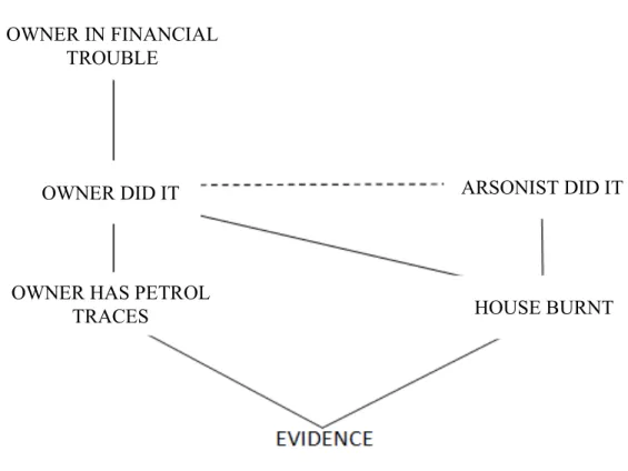
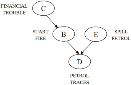
Figure 1 depicts the simple network that evaluates competing explanations in the house fire example. It includes a unit called OWNER IN FINANCIAL

(29)

TROUBLE that represents the hypothesis that the house owner was in financial trouble, and a unit called OWNER HAS PETROL TRACES that represents the evidence that the house owner had petrol traces on his clothes. The excitatory links between units representing coherent propositions and the inhibitory links between units representing incoherent propositions. In simulations, the links have different weights that can represent the degree of coherence or incoherence between propositions.

Figure 1. Neural network modelling competing explanations for the burning down of a house. The straight lines indicate coherence relations (positive constraints) established because a hypothesis explains a piece of evidence. The dotted lines indicate incoherence relations (negative constraints).

OWNER DID IT ARSONIST DID IT

HOUSE BURNT OWNER IN FINANCIAL

TROUBLE

OWNER HAS PETROL TRACES

(30)

Thagard’s theory (through ECHO) has been used to model some prominent jury verdicts (e.g. Thagard, 1989) and does much by way of solving some of the problems which beset coherence theories of justification, including coherence theories of legal justification (see Amaya, 2007). However, it still has a fundamental limitation. Lagnado (2011) has argued that coherence models are unable to represent basic forms of inference such as ‘explaining away’ (Pearl, 1988).

Explaining Away

Explaining Away is a common and intuitively compelling pattern of inference that refers to the idea that because one cause explains the observed effect it therefore reduces the need to invoke other causes. Wellman and Henrion (1993) illustrate this with the following example. A friend sneezes and this raises the probability of him having a cold, and the probability of him having an allergic reaction. Once it is found out that the friend is allergic to cats, and a cat is observed to be present, this lends confirmation to the hypothesis he is having an allergic reaction. This explains away the sneezing and, therefore, reduces the probability of the cold. In other words the two hypotheses were independent when the status of the evidence was unknown, but become conditionally dependent given its status.

This pattern of inference is naturally captured using a Bayesian Network representation. Bayesian networks have well-established foundations in probability theory, and are currently applied in many practical contexts. Bayesian networks consist of two parts: a graph structure and a set of conditional probability tables. The graph structure is made up of a set of nodes corresponding to the variables of interest, and a set of directed links between these variables corresponding to causal relations. The variables tend to be causes and effects but they could even be hypotheses about

(31)

pieces of evidence (such as in legal contexts). This yields a directed graph that represents the probabilistic relations between variables, in particular the conditional and unconditional dependencies. In addition to the graph, a Bayesian network also requires a conditional probability distribution table for each variable. This dictates the probability of the variable in question conditional on the possible values of its parents (the nodes with direct links into that variable). This arrangement of nodes and links, plus the conditional probability tables for each node, dictate what inferences are licensed (via the laws of probability).

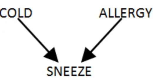
In a simplified model, there are three binary variables, Cold (C) which represents whether or not someone has a cold, Allergy (A) which represents whether or not someone has an allergy, and Sneeze (S) which represents whether or not someone sneezes. Both C and A are potential causes of S. The graph structure is depicted in Figure 2. This encodes the assumption that C and A are marginally independent, i.e., P(C) = P(C|A). The observation of sneezing raises the probability of both C and A: P(C|S) > P(C); P(A|S)>P(A). However, on observing that A is true, the probability of C returns to its prior level: P(C|A&S)=P(C). This is the basic phenomena of explaining away.

Figure 2. Graph structure for simple example of explaining away.

To understand how coherence models cannot cope with such a causal network it is sufficient to look at the way they would represent a simple criminal scenario.

(32)

Returning to the ‘house fire’ example, there could be two potential explanations for the petrol traces evidence: i) the petrol traces are from the petrol used to start the fire, or ii) the petrol traces are the result of the house owner spilling petrol while filling up his car. According to the first explanation the probability that the house owner is guilty is raised whilst according to the second explanation the probability of guilt is lowered. General coherence models assume that if two propositions both explain a piece of evidence, but they are not explanatorily connected, then the two propositions are incoherent with each other. This is expressed explicitly in Thagard’s ‘competition’ principle: if P and Q both explain a proposition, and if P and Q are not explanatorily connected, then P and Q are incoherent with each other.

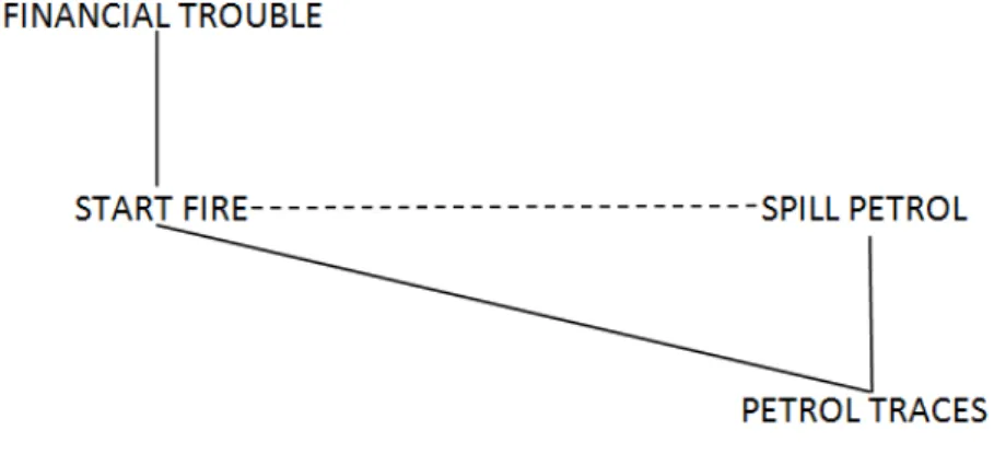
Returning to the house fire scenario example, the hypothesis that the owner spilled petrol while filling up his car, and the hypothesis that the owner has petrol traces on clothes because he started a fire, independently explain evidence and would therefore be treated as competitors that are incoherent with each other. However, this is an inappropriate representation of their true relation in the world. Whether or not the suspect spilled petrol while filling up his car is unrelated (independent) of whether or not he is guilty of starting the fire. The two explanations only become dependent given the evidence of petrol traces on the clothes that they both try to explain. This is clear by looking at Figure 3. It depicts the neural network that evaluates competing explanations for the petrol traces, as modelled by coherence accounts. Solid lines are excitatory links between units, and the dotted line is an inhibitory link representing incoherence between competing hypotheses about the origin of the petrol traces— starting a fire or spilling it while filling up car.

(33)

Figure 3. Connectionist network modelling competing explanations for petrol traces. 2.2 Experiment 1

The aim of this study was to show that mock jurors reason through crime scenarios by constructing causal networks that allow them to perform explaining away inferences that cannot be accounted for by coherence models. This was done by presenting participants with two fictional criminal scenarios based on a simple causal network that involved an explaining away causal inference.

Both scenarios began with background details about the crime and the chief suspect. Participants were then asked to make two baseline judgments. The first one was an estimate of the likelihood that the suspect was guilty (guilt judgment). The second one was an estimate of the likelihood of another event that might have caused the suspect to commit the crime (causal judgment). Once participants made these judgments they were presented with a new piece of evidence that incriminated the suspect (affirmative evidence) and were asked to make the same two judgments again. Lastly, they were presented with a new piece of evidence that explained away the previous piece of affirmative evidence (rebuttal evidence). Finally participants were asked to make the same judgments again. Participants thus gave six sequential

(34)

probability judgments in each problem (two baseline, two after affirmative evidence and two after rebuttal evidence).

This causal network is best explained using one of the crime scenarios as an example. The first scenario provided participants with the following background information: ‘A house burnt down. The police investigation reveals that the fire was caused by ignited petrol and was therefore intentional. Statistics show that in about half of cases of intentional burning down of houses, it is the owner who is responsible for starting the fire to get compensation money from insurance.’ Participants were then asked to make two baseline judgments. The first one was an estimate of the likelihood that the house owner was guilty (guilt judgment). The second one was an estimate of the likelihood that the owner was in financial trouble (causal judgment). After participants made their judgments they were provided with new affirmative evidence: ‘Further police investigation revealed that the owner had petrol traces on his clothes.’ Participants were then asked to make the same judgments as before. Next, participants were presented with a piece of rebuttal evidence which ‘explained away’ the piece of affirmative evidence: ‘Further police investigation revealed CCTV footage of the owner filling up his car with petrol and spilling petrol on his clothes.’ Finally participants were asked to make the two judgments one last time.

In contrast to the network representation suggested by the coherence approach (Figure 3), participants were hypothesised to have constructed a causal model that allowed for ‘explain away’ inferences. This is displayed in Figure 4.

(35)

Figure 4. Causal network for house fire scenario. The experimental hypotheses were:

i) guilt judgments after the affirmative evidence will be greater than the baseline judgments, showing that the affirmative evidence did in fact have the intended incriminating impact;

ii) causal judgments will also be greater after the affirmative evidence as participants create a causal link between the evidence and the causal judgment; iii) guilt judgments after the rebuttal evidence will be lower than the judgments

given after the affirmative evidence judgments, showing that participants make explaining away inferences;

iv) causal judgments will also be lower than the judgments given after the affirmative evidence because participants extend explaining away inferences to causal judgments.

The causal network in question and the relative hypotheses can also be expressed probabilistically (note that letter ‘A’ stands for the background evidence):

(36)

ii) P(C|A) > P(C| A&D);

iii) P(B| A & D) > P(B|A & D & E); iv) P(C| A & D) > P(C|A & D & E).

In order to assess whether participants had constructed the hypothesised causal model, they were presented with a series of questions that aimed to assess their causal schemas. In accordance it was hypothesised that participants would represent:

i) the guilt variable to be positively linked to the causal variable; ii) the guilt variable to be positively linked to the affirmative evidence; iii) the rebuttal evidence to be positively linked to the affirmative evidence iv) No link between the causal variable and the rebuttal evidence.

Importantly, the fourth hypothesis (stating the absence of a causal link between the casual variable and the rebuttal variable), directly assessed whether participants constructed an inhibitory link between the two alternative explanations for the evidence. Results supporting the experimental hypothesis would speak strongly against a coherence model based representation of the evidential reasoning.

2.3 Method Participants and Apparatus

65 first year undergraduate students from UCL (University College London) participated in the study in return for course credit. 52 participants were female and the mean age was 18.9 (1.47). The experiment was conducted online on individual computers and programmed in Adobe Dreamweaver.

(37)

Design

The experiment followed a within-subject design where each participant was presented with both scenarios. The order of the two scenarios was counterbalanced.

Materials and Procedure

The materials consisted of two scenarios. : the ‘House fire scenario’ and the ‘Injured child scenario’. Each scenario was accompanied by a set of judgment questions and ended with four causal questions

Scenarios and judgment questions

These are reported in Table 1 along with the questions, in the same order they were presented during the study. Both scenarios began with background details about the crime and the chief suspect. This simple description was followed by two questions: the baseline guilt judgment and the baseline causal judgment. Participants indicated their judgments on a slider scale that was labeled as from ‘extremely unlikely’ to ‘extremely likely’. The label in the center read ‘as likely as not’. This is shown in Figure 5. The scale did not have any numbers, but the responses were coded from 0 to 100 (with 0 = extremely unlikely, 50 = as likely as not, and 100 = extremely likely).

(38)

Table 1.

Table displaying the material shown to participants in the order in which it was presented. Experiment 1.

Scenario House fire Child

Background details

A house burnt down. The police investigation reveals that the fire was caused by ignited petrol and was therefore intentional.

Statistics show that in about half of cases of intentional burning down of houses, it is the owner who is responsible for starting the fire to get compensation money from insurance as they are in financial trouble.

A child who has been brought into hospital has serious head trauma related injuries. Medical and police records show that about half of children with those specific injuries have been violently shaken by their parents.

Baseline guilt judgement

Please indicate how likely it is that the owner was the one who burnt down the house.

Please indicate how likely it is that the child has been violently shaken. Baseline

causal judgment

Please indicate how likely it is that the owner was in financial trouble.

Please indicate how likely it is that the parents have mental health problems.

Affirmative evidence

Further police investigation revealed that the owner had petrol traces on his clothes.

Further police investigation revealed that the injuries presented by the child included retinal haemorrhages – a characteristic symptom of violent shaking.

Affirmative guilt judgement

In light of this new evidence please indicate how likely it is that the owner was the one who burnt down the house.

In light of this new evidence please indicate how likely it is that the child has been violently shaken.

Affirmative causal judgment

In light of this new evidence please indicate how likely it is that the owner was in financial trouble.

In light of this new evidence please indicate how likely it is that the parents have mental health problems.

Rebuttal evidence

Further police investigation revealed CCTV footage of the owner filling up his car with petrol and spilling petrol on his clothes.

Further police investigation revealed that the child was born with a severe vitamin C deficiency which causes retinal haemorrhages.

Rebuttal guilt judgement

In light of this new evidence please indicate how likely it is that the owner was the one who burnt

In light of this new evidence please indicate how likely it is that the child has been violently shaken.

Rebuttal causal judgment

In light of this new evidence please indicate how likely it is that the owner was in financial trouble.

In light of this new evidence please indicate how likely it is that the parents have mental health problems.

(39)

Participants were then presented with a piece of affirmative evidence that incriminated the suspect. Following this new information they were asked to repeat the two judgments (affirmative guilt judgment and affirmative causal judgment). Next they were presented with a piece of rebuttal evidence that discredited the affirmative evidence – it explained it away. Finally participants were asked to make the last two judgments: rebuttal guilt judgment and rebuttal causal judgment.

Causal questions

Four questions were constructed for each scenario to assess the causal model participants had constructed. Each question consisted in a forced choice question (these are reported in Table 2) and a confidence judgment. The confidence judgment consisted in a likelihood rating.

Table 2.

Table showing the causal questions for each scenario. Experiment 1.

Scenario House fire Child

Causal question 1

Do you think knowing a suspect might be in financial trouble is relevant to whether the suspect burnt down his house?

Do you think knowing that suspects might have mental health problems is relevant to whether the suspects are responsible for violently shaking their child?

Causal question 2

Do you think knowing a suspect has petrol traces on his clothes is relevant to whether the suspect burnt down his house?

Do you think knowing a child has retinal haemorrhage is relevant to whether the child has been violently shaken?

Causal question 3

Do you think knowing a suspect has spilt petrol on his clothes while filling up his car is relevant to knowing the suspect has petrol traces on his clothes?

Do you think knowing a child has vitamin C deficiency is relevant to knowing the child has retinal haemorrhage?

Causal question 4

Do you think knowing a suspect might be in financial trouble is relevant to knowing the suspect has spilt petrol on his clothes while filling up his car?

Do you think knowing suspects might have mental health problems is relevant to knowing their child has vitamin C deficiency?

(40)

The reason why the ‘Equally likely option’ was not given as a possible answer in the forced choice question, was to tackle the worry that participants might select it to remain neutral (avoid giving a wrong answer) rather than to indicate actual feeling that the connections are indeed equally likely. For this reason the forced choice question was followed by a confidence judgment. It was presumed that participants who constructed a causal link would give a higher likelihood rating whereas participants who did not construct a causal link (i.e. thought the two answers were equally likely) would select one of the answers and then give the lowest likelihood rating. For example, to assess the presence of a positive causal link between the guilt variable and the casual variable in the ‘Injured child scenario’, participants were asked:

Which parents are more likely to violently shake their child?

o Parents with mental health problems

o Parents without mental health problems

How much more?

Figure 6. Response scale for the causal questions

2.4 Results Scenario judgments

The mean and standard deviation of the three sets of guilt and causal judgments are displayed in Table 3.

(41)

Table 3.

Mean and standard deviation of guilt judgments and causal judgments. Experiment 1. House fire scenario Injured child scenario

Judgment Guilt Causal Guilt Causal

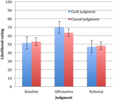
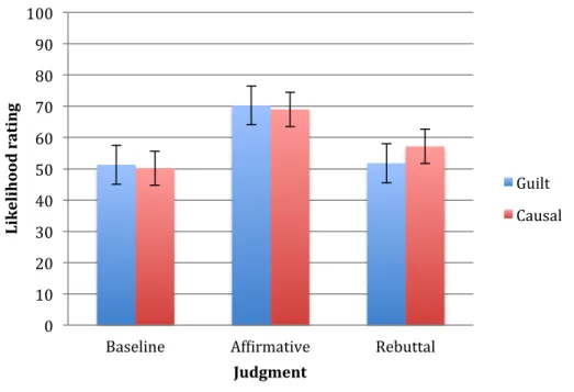
Baseline 51.4 (9.8) 52.9 (11.6) 51 (10.3) 47.3 (16) Affirmative 69.8 (12.4) 63.5 (13.6) 73.2 (12.3) 59.7 (19.9) Rebuttal 46.9 (14.3) 48.1 (14.6) 41.7 (13.4) 42 (13.8)

T-tests

Paired samples t-tests were conducted to evaluate the significance of the results. The way the judgments change after the affirmative and rebuttal evidence is clear by observing Figure 6 (House fire scenario) and Figure 7 (Injured child scenario)

House fire scenario. The first hypothesis was supported as there was a significant increase between guilt judgments given at baseline and those given after the affirmative evidence: t(64)= -8.89, p<0.001. The same was true for causal judgments (hypothesis 2): t(64)= -4.48 p<0.001. Also supported was the third hypothesis, which predicted that participants’ guilt judgments given after the rebuttal evidence would be significantly lower than the ones given after the affirmative evidence: t(64)=9.151, p<0.001. The same was true for causal judgments (hypothesis 4) t(64)=6.144, p<0.001.

Interestingly, inspection of the means and graph showed participants’ guilt and causal judgments given after the rebuttal evidence were both lower than the initial baseline judgments. A paired sample t-test was conducted to evaluate whether there was a significant difference between the rebuttal guilt judgment and the baseline guilt judgment. The result was indeed significant, t(64)=2.218, p=0.03. The same was true for the difference between the rebuttal causal judgment and the baseline causal judgment, t(64)=2.18, p=0.033.

(42)

Injured child scenario. The first hypothesis was supported as there was a significant increase between guilt judgments given at baseline and those given after the affirmative evidence: t(64)= -10.8, p<0.001. The same was true for causal judgments (hypothesis 2): t(64)= -3.9 p<0.001. Also supported was the third hypothesis, which predicted that participants’ guilt judgments given after the rebuttal evidence would be significantly lower than the ones given after the affirmative evidence: t(64)=14.9, p<0.001. The same was true for causal judgments (hypothesis 4) t(64)=5.54, p<0.001.

Interestingly, inspection of the means and graph showed participants’ guilt and causal judgments given after the rebuttal evidence were both lower than the initial baseline judgments. A paired sample t-test was conducted to evaluate whether there was a significant difference between the rebuttal guilt judgment and the baseline guilt judgment. The result was indeed significant, t(64)=-4.286 p<0.001. On the other hand, the difference between the rebuttal causal judgment and the baseline causal judgment was not signficiant, t(64)=-1.86, p=0.067.

(43)

Figure 6. Graph showing the mean guilt and causal judgments (with error bars). Experiment 1, ‘House Fire’ scenario.

Figure 7. Graph showing the mean guilt and causal judgments (with error bars). Experiment 1, ‘Injured child’ scenario.

0 10 20 30 40 50 60 70 80 90 100

Baseline Af@irmative Rebuttal

Li k el ih oo d r at in g Judgment Guilt judgment Causal judgmemt 0 10 20 30 40 50 60 70 80 90 100

Baseline Af@irmative Rebuttal

Li k el ih oo d r at in g Judgment Guilt judgment Causal judgmemt

(44)

ANOVAs

House Fire scenario. A one-way repeated measures ANOVA was conducted to compare the guilt judgments given at the three different stages (after background evidence, after affirmative evidence and after rebuttal evidence). There was a significant effect for guilt judgment, Wilk’s Lambda = 0.388, F (2, 63) = 49.6, p < 0.001, multivariate partial eta squared = 0.61. Post hoc tests using the Bonferroni correction revealed that, in line with the results obtained from the paired t-tests, affirmative judgments were significantly higher than baseline judgments (p<0.001) and that rebuttal judgments were significantly higher than affirmative judgments (p<0.001). On the other hand, the rebuttal judgments were not significantly lower than baseline judgments (p=0.09).

A very similar pattern of results is revealed by running the one-way repeated measures ANOVA on the causal judgments. There was a significant effect for guilt judgment, Wilk’s Lambda = 0.624 F (2, 63) = 19.001 p < 0.001, multivariate partial eta squared = 0.376. Post hoc tests using the Bonferroni correction revealed that, in line with the results obtained from the paired t-tests, affirmative judgments were significantly higher than baseline judgments (p<0.001) and that rebuttal judgments were significantly higher than affirmative judgments (p<0.001). On the other hand, the rebuttal judgments were not significantly lower than baseline judgments (p=0.099).

Injured child scenario. The same analyses were repeated for the ‘Injured child’ scenario. A one-way repeated measures ANOVA was conducted to compare the guilt judgments given at the three different stages (after background, after affirmative evidence and after rebuttal evidence). The was a significant effect for guilt judgment, Wilk’s Lambda = 0.209, F (2, 63) = 119.22, p < 0.0001, multivariate partial

(45)

eta squared = 0.791. Post-hoc tests using the Bonferroni correction revealed that, in line with the results obtained from the paired t-tests, affirmative judgments were significantly higher than baseline judgments (p<0.001) and that rebuttal judgments were significantly higher than affirmative judgments (p<0.001). Additionally, the rebuttal judgments were significantly lower than baseline judgments (p<0.001).

A very similar pattern of results is revealed by running the one-way repeated measures ANOVA on the causal judgments. The was a significant effect for guilt judgment, Wilk’s Lambda = 0.409 F (2, 16) = 11.551 p < 0.001, multivariate partial eta squared = 0.591. Post hoc tests using the Bonferroni correction revealed that, in line with the results obtained from the paired t-tests, affirmative judgments were significantly higher than baseline judgments (p<0.001) and that rebuttal judgments were significantly higher than affirmative judgments (p=0.038). On the other hand, the rebuttal judgments were not significantly lower than baseline judgments (p=0.202).

Individual analyses

Individual differences in patterns of responses were analyzed for both sets of judgments. Table 4 shows the number (and percentage) of participants who: i) gave affirmative judgments greater than baseline judgments; ii) gave rebuttal judgments lower than affirmative judgments; gave all judgments consistent with the hypotheses; and iv) participants who did not over-adjust the rebuttal judgment to be lower than baseline.

(46)

Table 4.

Table showing individual differences in judgment patterns. Experiment 1.

House fire scenario Injured child scenario

Judgment Guilt Causal Guilt Causal

Baseline > Affirmative 57 (88%) 49 (75%) 60 (92%) 43 (66%) Affirmative < Rebuttal 57 (88%) 51 (78%) 60 (92%) 53 (82%) Baseline > Affirmative < Rebuttal 54 (83%) 42 (65%) 57 (88%) 36 (55%) Baseline < Rebuttal 23 (35%) 26 (40%) 20 (31%) 28 (43%)

Causal Model assessment

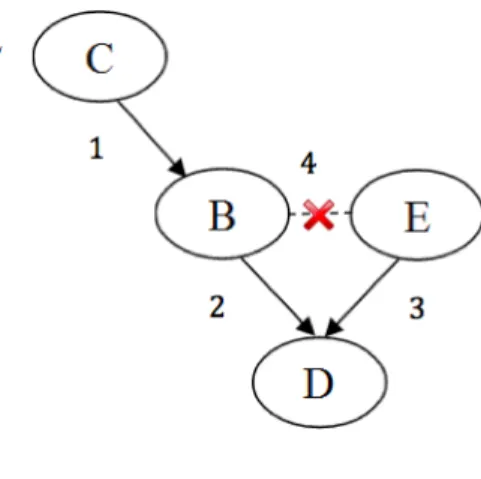
Figure 7 shows the hypothesized causal model for the two scenarios. Table 5 shows the percentage of participants who constructed each link (this was calculated based on the forced choice question. It is the number of participants who responded that a link between the two entities was more likely). The table also shows the mean confidence rating for each participant.

Figure 7. The hypothesized causal model for the two scenarios (C=causal variable; B=guilt variable; E=rebuttal evidence; D=affirmative evidence). The crossed dashed line indicates the absence of the incoherence link. The numbers correspond to the data in the table 5 below.