2017 2nd International Conference on Communications, Information Management and Network Security (CIMNS 2017) ISBN: 978-1-60595-498-1
Stopout Research Based on Behavior in Massive Open Online Courses
Wen YIN, Ming-hua JIANG
*, Chang-long ZHOU and Li-ling ZHOU
Wuhan Textile University, Wuhan, China *Corresponding author
Keywords: MOOC, Stopout, Behavior, Predicted, Logistic regression.
Abstract. In recent years, the loss of a large number of learners has attracted widespread attention in Massive Open Online Courses (MOOCs). A great deal of research has been modeling analysis and predicted based on the learning behavior. In this paper, according to the modules provided by moocroom, extract some related behavior, select the learners registered after the first three weeks of the data as the data set, using logistic regression modeling analysis, forecast for the next few weeks whether learners stopout, final assessment of the model performance. Experimental results indicate that the model established achieves high prediction accuracy, and the models attained the average AUC is 0.76.
Introduction
With the recent boom in development of Massive Open Online Courses (MOOCs), as a new form of online teaching has gained enormous popularity and attention. However, against a background of thriving enrollment, the completion rate of MOOCs is staggeringly low [1],[6]. So more concern is that the significant decrease in participation. Previous research indicates that fewer than 7% of learners who enroll in a MOOC actually complete it [2]. Learner stopout usually takes place by the second week of the course [3]. There are relevant research have analyzed the cause of stopout [4],[5]. One reason is that the online learning teachers can't see the learning situation of the learners in time, and the teachers can't get the learning feedback as the face-to-face teaching.
By analyzing the behavior of learners [7], it can well reflect the purpose, status and habits of learners, and provide effective feedback for teachers. This feedback allows the teacher to adjust the course in a timely manner to suit the learners' rhythm. A potential interaction between teachers and students is achieved. It can not only improve the experience of MOOC, but also improve the learning efficiency.
In this paper, We put the moocroom[10] (A MOOC platform) learners as the research object, according to the specific function module extraction behavior of moocroom, using logistic regression to learn the first three weeks of the conduct of the modeling and analysis, predict whether learners stopout in the next 7 weeks and the average weight of various feature.
The remainder of this paper is organized as follows: A brief description of four types of behavior in moocroom is in Section 2. Training and evaluation models are presented by logistic regression in Section 3. The experiment results and evaluation through training is illustrated in Section 4. Finally, Section 5 concludes the paper.
Behavior Features in Moocroom
According to the activity frequency of each module in the moocroom, the learner activity can be divided into four categories: explore behavior, course behavior, interactive behavior and other behaviors.
1. exploring behavior: Look for courses you want to study or browse through a circle of interest in moocroom.
2. course behavior: the learner and the specific course learning related behavior. 3. interaction behavior: The interaction between a learner and a teacher or platform
Figure 1 shows the proportion of four types of behavior. Course behavior accounts for the largest proportion, It shows that the core of MOOC is the part of the course that best reflects the learner's motivation, purpose, status and habits. Therefore, this paper will extract the learner's behavioral features from the course behavior as model input.
Figure 1. The proportion of four types of behavior.
Predicting Stopout Base on Course Behavior
We made several assumptions to more precisely define the stopout prediction problem and interpret the data. These assumptions include time-slice delineation and defining persistence (stopout) as the event we attempt to predict.
1. Time-slice and Stopout definition
Temporal prediction of a future event requires us to assemble explanatory variables along a time axis. This axis is subdivided to express the time-varying behavior of variables so they can be used for explanatory purposes. we decided to define weekly units as time slices. The duration of observation was 10 weeks after registration.
The next question we had to address was our definition of stopout. We considered defining it by the learner’s last behavior in the course, regardless of the nature of the course. In any given week, the learner displays any course behavior and judges that the learner has persistence. Determining a learner's stopout means not showing any learning behavior during the week, such as logging in, but without any course behavior or no login.
2. Features per learner
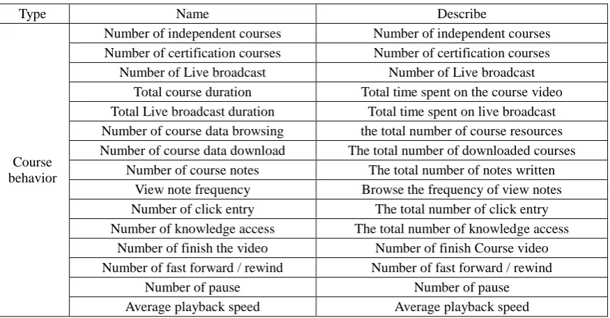
[image:2.595.81.519.568.796.2]We extracted 15 interpretive features on a per-learner basis. These are the features we use to build a model. In this paper for the sake of brevity, we only list the features and their brief descriptions in the Table 1.
Table 1. Self-extracted covariates.
Type Name Describe
Course behavior
Number of independent courses Number of independent courses Number of certification courses Number of certification courses
Number of Live broadcast Number of Live broadcast Total course duration Total time spent on the course video Total Live broadcast duration Total time spent on live broadcast Number of course data browsing the total number of course resources Number of course data download The total number of downloaded courses
Number of course notes The total number of notes written View note frequency Browse the frequency of view notes Number of click entry The total number of click entry Number of knowledge access The total number of knowledge access
Number of finish the video Number of finish Course video Number of fast forward / rewind Number of fast forward / rewind
Number of pause Number of pause
The course behavior is represented by the C, so the explanatory variables are represented by C1, C2,..., and Cn.
Training
Logistic regression is a commonly used binary predictive model. It calculates a weighted average of a set of variables, submitted as covariates, as an input to the logit function. Thus, the input to the logit function, Z, takes the following form:
Z=a0+a1*X1+a2*X2+...+an*Xn (1)
Here, a1 to an are the coefficients for the feature values, X1 to Xn. a0 is a constant. The logit
function, given by,
g(z) = yi = 1
1+e−z (2)
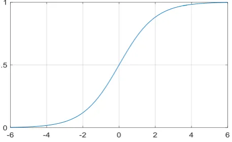
[image:3.595.185.414.290.430.2]takes the shape as shown in figure 2. Note that the function’s range is between 0 and 1, which is optimal for probability. Also note that it tends to ‘smooth out’ at extreme input value, as the range is capped.
Figure 2. The logit (aka logistic or sigmoid) function.
For a binary classification problem, such as ours, the output of the logit function becomes the estimated probability of a positive training example. These feature weights, or coefficients, are similar to the coefficients in linear regression. The difference is that the output ranges between 0 and 1 due to the logit function, rather than an arbitrary range for linear regression.
Corresponding binary label associated with the covariates. After training a model, the predicted probability, or the output of the logit function, should predict higher probabilities for the positive ‘+1’ class examples in the training data and a lower probability for the negative ‘0’ class examples.
There is no closed form solution to find the optimal coefficients to best fit the training data. As a result, training is usually done iteratively through a technique called maximum likelihood estimation. First, a random set of coefficients are chosen. At each iteration, an algorithm such as Newton’s method is used to find the gradient between what the coefficients predict and what they should predict, and updates the weights accordingly. The process repeats until the change in the coefficients is sufficiently small. This is called convergence. After running this iterative process over all of the training examples, the coefficients represent the final trained model.
Evaluation
With training in place, the next step is evaluating the classifier’s performance. A testing set comprised of untrained covariates and labels evaluates the performance of the model on the test data following the steps below:
1. The logistic function learned and presented in (2) is applied to each data point and the estimated probability of a positive label y𝑖 is produced for each data point in test set.
g(z)={1, if yi ≥ ℷ
0, if yi ≤ ℷ (3)
Given the estimated labels for each data point g(z) and the true labels. We can calculate the confusion matrix, true positives and false positives and thus obtain an operating point on the ROC curve.
3. By varying the threshold λ in (3) the decision rule above we can evaluate multiple points on the ROC curve. We then evaluate the area under the curve and report that as the performance of the classifier on the test data.
Prediction Result and Evaluation
We applied logistic regression to student persistence prediction. We used the 15 interpretive features we described earlier in this paper to form the feature vectors, and maintained the stopout value as the label.
C1,C2, ,Cn
C1,C2, ,Cn C1,C2, ,Cn
Logistic regression
the optimal parameters
prediction model
Z=a0+a1*C1+a2* C2+...+an* Cn
Maximum Likehood Estimate
g(z)=1/1+e-z
W1 W2 Wm
S=0
S=1 g(z)>λ g(z)<λ
C1,C2, ,Cn
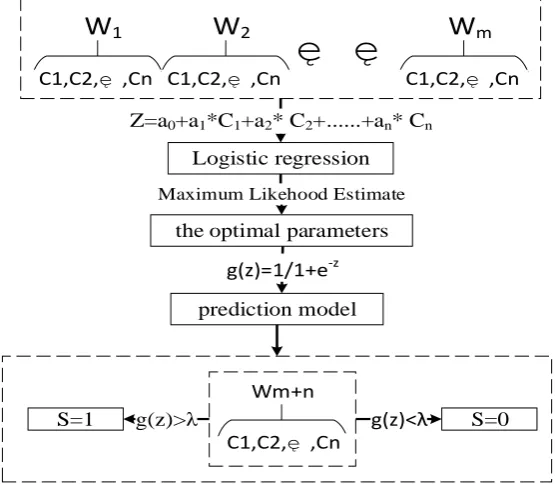
[image:4.595.159.437.262.504.2]Wm+n
Figure 3. The dashed part represents the feature matrix(Wm), which captures each feature value for each week. Each student has such a matrix.
According to figure 3, take m=3, the flow is as follows:
1. Performed 10 fold cross validation on the training set. This involved training the model on 9 folds of the train dataset and testing on the last fold.
2. Trained a logistic regression model on the entire train dataset.
3. Applied the model to the test dataset by putting each data point through the model then applying the decision rule in (3) and following the steps to determine the AUC under the ROC.
Figure 4. The average weight of feature.
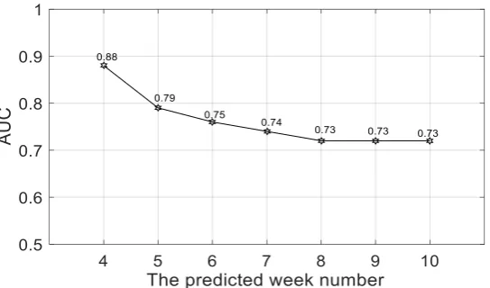
Figure 5. How the AUC varied as the target prediction week changed.
Conclusion
In Figure 4, these three factors (C4/Total course duration, C5/Total Live broadcast duration, C12/Number of finish the video) have a greater impact on whether learners have stopout in the next few weeks. In Figure 5, the maximum AUC is 0.88, and the average AUC is 0.76, which shows that the model is feasible for prediction classification. With the increase of the predicted week number, AUC will decrease. It shows that the model is better for short-term prediction. Of course, there are many parts of this paper that have not been investigated. Will it be better to use more historical data modeling? Or different models such as Hidden Markov model [8]? Whether the model applies to a different discipline, a different context, or a different MOOC platform [9]?
References
[1] Ho A D, Reich J, Nesterko S O, et al. HarvardX and MITx: The first year of open online courses, fall 2012-summer 2013[J]. 2014.
[2] Parr C. New study of low MOOC completion rates| Inside Higher Ed[J]. Inside Higher Ed, 2013.
http://www.insidehighered.com/news/2013/05/10/new-studylow-mooc-completion-rates?utm_sourc e=feedly.
[image:5.595.159.431.286.446.2][4] Willging P A, Johnson S D. Factors that influence students' decision to dropout of online courses[J]. Journal of Asynchronous Learning Networks, 2009, 13(3): 115-127.
[5] Boyer S S A. Transfer learning for predictive models in MOOCs[D]. Massachusetts Institute of Technology, 2016.
[6] Han F. Modeling Problem Solving in Massive Open Online Courses[D]. Massachusetts Institute of Technology, 2014.
[7] Boyer S S A. Transfer learning for predictive models in MOOCs[D]. Massachusetts Institute of Technology, 2016.