Dynamic Evaluation on the Groundwater Flow Process in a River Basin Using the Ensemble Kalman Filter Method with Localization

2016 International Conference on Mathematical, Computational and Statistical Sciences and Engineering (MCSSE 2016) ISBN: 978-1-60595-396-0

Dynamic Evaluation on the Groundwater Flow Process in a River Basin

Using the Ensemble Kalman Filter Method with Localization

Liang XUE

Department of Oil-Gas Field Development Engineering, College of Petroleum Engineering, China University of Petroleum, 18 Fuxue Road, Changping District, Beijing, China 102249

*Corresponding author

Keywords: Stochastic analysis, Inverse modeling, Ensemble kalman filter, Localization function.

Abstract. Ordos Plateau is located in a semi-arid area in the northwest part of China, and groundwater water is the major water source to sustain the ecosystem. With the industrial construction and economic development, it is required to manage the groundwater usage reasonable. Several monitoring instruments have been installed to monitor the groundwater dynamics continuously. An ensemble Kalman filter based data assimilation method is developed to use the sequentially available monitoring data to characterize the groundwater system. To improve the algorithm stability and avoid the spurious correlation estimation, a localization function is introduced. The analysis results show the proposed EnKF method can reduce the estimation uncertainty and improve the predictability.

Introduction

Vast reserves of mineral resources, such as petroleum, natural gas, coal and halite, have been found in the Ordos Plateau in the northwest part of China. With the development of industrial infrastructure construction, agriculture and urbanization, the demand for water resources increases rapidly. However, this region is located in an arid or semi-arid area with the groundwater as the main source for water supply. Groundwater resources are critical to sustain the local fragile ecological environment. Overexploitation of groundwater may cause severe ecological damage to this area, which may reversely affect the local economic growth in the long run. To improve the groundwater resources management, it is essential to understand the groundwater dynamics accurately and make a reasonable plan on the groundwater usage.

Groundwater modeling is an effective quantitative tool to predict the groundwater system behavior. It requires a set of model parameters to characterize the physical properties of groundwater system. However, groundwater system is a complex natural system. System properties may vary dramatically in space, such as hydraulic conductivity and porosity, which makes it difficult to fully characterize the heterogeneity of the system parameters. Consequently, substantial uncertainties are associated with the prediction of system behavior in groundwater system. Stochastic analysis method has been introduced by researchers to perform groundwater modeling to cope with this issue [1,2,3,4,5].

To constrain the system parameters and reduce the uncertainty associated with the prediction, stochastic inverse modeling has become an active research topic [6,7,8,9]. It serves as a method to use measurement data to estimate the model parameters. With the deployment of the real-time sensors in the Ordos Plateau to monitoring the groundwater level fluctuation, it is required to develop a theoretical framework which has the capability to take advantage of the available monitoring data to improve the characterization of the groundwater system and aid the decision-making on the ecological system protection during the industrial construction process in this region.

parallel computing since the model evaluation for a specific ensemble member does not interact with others, which is a notable feature especially for the large scale numerical model that is time consuming to evaluate.

The aim of paper is to develop a stochastic analysis framework for data assimilation suitable to the data collected from the groundwater monitoring technique available in this region to analyze the groundwater dynamics using the EnKF method. This paper is organized as follows: Section 2 introduces the numerical model for the research area and the theoretical background of the EnKF with localization; Section 3 demonstrates the procedures and results to assimilate the groundwater level data to characterize the heterogeneous hydraulic conductivity field; Conclusions are drawn and future work is suggested based on the analysis results in Section 4.

Methodology

Site Description

Hailiutu river basin is located in the northwest part of China, as shown in Figure 1. It is a sub-region of the Ordos plateau with an area of 2600 Km2. Notable agricultural activities and natural gas productions occur in this area, which demands a large amount of groundwater extraction. The average annual precipitation is about 380mm which mostly occurs from March to October, but the average annual potential evaporation is around 1900mm. This indicates that Hailiutu river basin is in a semi-arid region. The groundwater fluctuation is controlled by these recharge and evaporation processes. To collect the information on the groundwater level fluctuation, several monitoring wells has been set in this area. Here, we select two monitoring wells, i.e., well 1 and 2 as shown in Figure 1, as data sources to perform data assimilation process, since these two wells can provide us consecutive data set for about 3 years.

Figure 1. The sketch map of Hailiutu river basin and the locations of monitoring wells.

approaching to the end. It is necessary to build a computational model with these two geological layers and the river system involved jointly.

Numerical Model

The numerical model of the groundwater system is built with the aid of MODFLOW software. It essentially uses the finite difference method to solve the partial differential equation that governs the groundwater flow.

In the unconfined flow problem under Dupuit assumption, it can be written as

     

 

 

K h t h t W t S

t



_  _ 

 x

x x x x (1)

In the confined flow problem, it can be written as

   

 

 

K h t W t S

t

 _  _ 

 x

x x x (2)

which is subject to the initial and boundary conditions,

( , 0) ( )

h x  x (3)

( , ) ( , ), _D

h xt  xt x (4)

 

K x h x t n x Q x t x (5)

where h is pressure head; K is the hydraulic conductivity; W is the source/sink term; Sy is the specific yield; Ss is the specific storage; is the initial head;  is the prescribed head on Dirichlet boundary

D

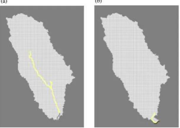
 ; Q is the prescribed flux on Neumann boundary _N; ( )n x is the outward vector normal to _N. The rectangular research area is discretized into 140 columns along the x-axis ranging from 290000m to 360000m, and 200 rows along y-axis ranging from 4210000m to 4310000m, which indicates that each cell covers an area of 500m×500m. The system boundary is extracted from a remote sensing image. The cells out of the boundary are deactivated (as the grey area shows in Figure 2) and 20840 active cells are involved in the computation process of groundwater flow.

Figure 2. Finite difference grid of the research area: (a) top layer, (b) bottom layer. The yellow line represents the Hailiutu river.

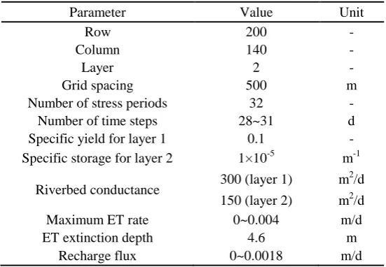
Table 1. Parameter values for groundwater modeling in Hailiutu river basin.

Parameter Value Unit

Row 200 -

Column 140 -

Layer 2 -

Grid spacing 500 m

Number of stress periods 32 -

Number of time steps 28~31 d

Specific yield for layer 1 0.1 -

Specific storage for layer 2 1×10-5 m-1

Riverbed conductance 300 (layer 1) m

2_/d

150 (layer 2) m2/d

Maximum ET rate 0~0.004 m/d

ET extinction depth 4.6 m

Recharge flux 0~0.0018 m/d

The EnKF with Localization

The EnKF method is derived on the basis of Kalman filter [13] by Evensen [14]. The EnKF method overcomes the underlying assumption of model linearity required by Kalman filter and estimate the covariance matrix of state vector through Monte Carlo simulation in an ensemble manner.

Define the ensemble of state vector as,





1 2 , , , ( ) ( ) ( ) ( ) ( ) _{( )} e e e e N N N N                Y Y Y

s s s M Y M Y M Y G Y G Y _{G Y}

(6)

where YlnK is the natural logarithm of hydraulic conductivity which is considered as a random variable due to the difficulty to characterize its spatial heterogeneity; G

 

model parameters with state vector; M( ) is the model operator which represents the groundwater flow model as shown by Eq. 1-5.

In the forecast step of the EnKF, the state vector is moved forward from time step t-1 to t.

 

, , 1 , 1, 2, ,

f u

i t  i t i Ne

s M s (7)

where f represents the forecast step; u represents the update step. The observation data d and the state vector s are related by

,

obs true i t  t  t

d Hs ε (8)

where H[ ]0 I is a transferring matrix with elements of 0 and 1; ε_t is the measurement error and usually assumed to be Gaussian-distributed with 0 mean and covariance

 

T

t t t

E ε ε Cd .

The ensemble mean and covariance of state vectors are:

, 1

1 Ne

f f

t i t

i e N 





s s (9)





f f f f f

t i t t i t t

N 

   

 _  _{ }  _





s

In the update step, the Kalman gain is required which is a weighting matrix acting on the innovation term (the difference between measurement and prior estimation in the forecast step),





, , ,

f T f T

t t t t t t t



 s s  d

K C H H C H C (11)

Since the EnKF uses the ensemble statistics to compute Kalman gain, there may be remarkable sampling errors associated with the computation due to the insufficiency of ensemble size. Consequently, it may generate spurious correlations for two distance points in the estimation of state vector covariance ,

f t

s

C and hence Kalman gain, which makes the EnKF numerically unstable. One

way to deal with this issue is to use localization [15], which introduces a distance-dependent localization function L to act on the state vector covariance:

1 1 11 1 1

1 1

( ) ( )

( ) ( )

s s

s s s s s s

N N f

s

N N N N N N

l c l c

L

l c l c

       _{  }  _{ }   

x x x x

C

x x x x

(12)

where is the elementwise Shur product.

In this case, the Kalman gain can be rewritten as,





, , ,

f T f T

t L t t tL t t t



  s  s  d

K C H H C H C (13)

The update state vector is:

, , , ,

u f obs f

i t  i t  t i t  t i t

s s K d H s (14)

After a set of trial tests, a piecewise localization function is chosen to help improving the EnKF stability for this case study.

5 4 3 2

5 4 3 2 1

1 1 5 5

1, 0

4 2 8 3

1 1 5 5 2

( ) 5 4 , 2

12 2 8 3 3

0, 2

x x x x

x

x x x x x x

L x x

x                 _{       }              _{ }  _{ }  _{ }  _{ }               _ _{ }  _{ }  _{ }  _{ }  _{ }  _{ }                    (15)

where  is the characteristic length. Here, it is set to be 3 times as long as the integral scale.

Result and Discussion

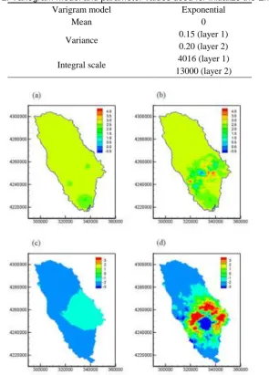
Table 2. Variogram model and parameter values used for initialize the EnKF.

Varigram model Exponential

Mean 0

Variance 0.15 (layer 1)

0.20 (layer 2)

Integral scale 4016 (layer 1)

13000 (layer 2)

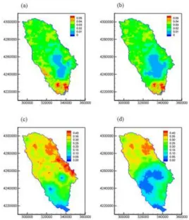
Figure 4. The ensemble variance of LnK: (a) initial, top layer; (b) updated, top layer; (a) initial, bottom layer; (b) updated, bottom layer.

Figure 3 and Figure 4 show the ensemble mean and variance of the random log hydraulic conductivity field in the initial step of the EnKF and these after 32-step updating using the EnKF method to assimilate the observed groundwater level data in the two monitoring wells. It can be found in Figure 3 that the ensemble mean of LnK value at the initial step (as shown by Figure 3(a) for top layer and Figure 3(c) for the bottom layer) is very smooth, even though they are conditional on 13 LnK measurement data. After 32 steps of data assimilation using the EnKF method, the heterogeneity of the estimated LnK field becomes better characterized as shown in Figure 3(b) for top layer and Figure 3(d) for the bottom layer, especially for the lower zone of the research area, which can be attributed to the fact that the monitoring wells are located in the corresponding lower zone. The ensemble variance distribution is shown in Figure 4. By comparing Figure 4(a) with Figure 4(b) for the top layer and Figure 4(c) with Figure 4(d) for the bottom layer, it can be observed that the blue zones around the location of monitoring wells are enlarged after the data assimilation process. It indicates that the estimation variance of the LnK field is reduced in these zones. The results show that the monitoring groundwater fluctuation data provide useful information to improve the LnK field estimation and reduce the corresponding estimation variance. The upper zone shows little change in either the ensemble mean (as shown in Figure 3) or ensemble variance (as shown in Figure 4). It is understandable because no monitoring well exists in the upper zone of the research area, and hence no information is available to update the field characterization. With the installment of more monitoring devices in this area, better estimation on the hydrogeological property can be expected.

information collected from the monitoring well are fully utilized to update the field characterization, and the LnK estimation is the most optimal relative to the current available information. It can improve the groundwater level prediction and more reasonable plan on the industrial development and ecological protection can be made by the government agency based on the data assimilation analysis result using the ensemble Kalman filter method.

Figure 5. Groundwater level in the initial step: (a) well 1, (b) well 2. Black curves (size of 100) represent the initial ensemble predictions, and red curve represents the measurement.

Figure 6. Groundwater level in the end of the updated step: (a) well 1, (b) well 2. Black curves (size of 100) represent the initial ensemble predictions, and red curve represents the measurement.

Summary

confirms that the ensemble Kalman filter method is an effective method to improve the hydrogeological field characterization and the corresponding groundwater fluctuation prediction. To avoid the failure of the state vector correlation estimation in the EnKF method, the localization function can be introduced. With more monitoring information available, field characterization can be continuously improved since the EnKF method is a sequential method.

Acknowledgements

This work is funded by the National Natural Science Foundation of China (Grant no. 41402199), the Science Foundation of China University of Petroleum, Beijing (Grant no. 2462014YJRC038), the independent research funding of State Key Laboratory of Petroleum Resources and Prospecting (Grant no. PRP/indep-4-1409) and the Platform Construction Project for Researches on the Relationship between Water and Ecology in the Ordos Plateau (Grant no. 201311076).

References

[1] A. A. Bakr, L. W. Gelhar, A. L. Gutjahr, J. R. MacMillan, Stochastic analysis of spatial variability in subsurface flows: 1. Comparison of one‐and three‐dimensional flows, Water Resources Research, 14 (1978) 263-271.

[2]G. Dagan, Stochastic modeling of groundwater flow by unconditional and conditional probabilities: 1. Conditional simulation and the direct problem, Water Resources Research, 18 (1982) 813-833.

[3] L. W. Gelhar, Stochastic subsurface hydrology from theory to applications, Water Resources Research, 22 (1986) 135-145.

[4] D. Russo, M. Bouton, Statistical analysis of spatial variability in unsaturated flow parameters, Water Resources Research 28 (1992) 1911-1925.

[5] D. Zhang, Stochastic methods for flow in porous media: coping with uncertainties, Academic press, 2001.

[6] J. Carrera, S. Neuman, Estimation of aquifer parameters under transient and steady state conditions: 1. Maximum likelihood method incorporating prior information, Water Resour. Res., 22 (1986) 199-210.

[7] B. S. Ramarao, A. M. LaVenue, G. de Marsily, M. G. Marietta, Pilot point methodology for automated calibration of an ensemble of conditionally simulated transmissivity fields, 1: Theory and computational experiments, Water Resour. Res., 31 (1995) 475-493.

[8] D. A. Zimmerman, et al., A comparison of seven geostatistically based inverse approaches to estimate transmissivities for modeling advective transport by groundwater flow, Water Resour. Res., 34 (1998) 1373-1413.

[9] H. J. Hendricks Franssen, A. Alcolea, M. Riva, M. Bakr, N. van der Wiel, F. Stauffer, and A. Guadagnini, A comparison of seven methods for the inverse modeling of groundwater flow: Application to the characterisation of well catchments, Adv. Water Resour., 32 (2009) 851-872.

[10] G. Burgers, P. van Leeuwen, G. Evensen, Analysis scheme in the ensemble Kalman filter, Mon. Weather Rev., 126 (1998) 1719-1724.

[11] Y. Gu, D. S. Oliver, The ensemble Kalman filter for continuous updating of reservoir simulation models, Trans. Soc. Mech. Eng. J. Energy Resour. Technol., 128 (2006) 79-87.

[13] R. E. Kalman, A new approach to linear filtering and prediction problems, J. Basic Eng., 82 (1960) 35-45.

[14] G. Evensen, Sequential data assimilation with a nonlinear quasigeostrophic model using Monte Carlo methods to forecast error statistics, J. Geophys. Res., 99 (1994) 10143-10162.