A Desk top tutorial Demonstration of Model based Fault Detection and Diagnosis

A Desk-top tutorial Demonstration of Model-based Fault Detection and

Diagnosis

John Z Shi1,2, Ali Elshanti2, Fengshou Gu2, and Andrew Ball2 1

School of Computing and Engineering, University of Huddersfield, HD1 3DH, UK Telephone: +44 1484 472842 Email: [email protected]

2

MACE, University of Manchester, M13 9PL, UK

Dr John Z Shi received the BSc degree in Mechanical Engineering and MSc degree in Mechatronic Engineering from Hebei University of Technology, Tianjin, China, in 1984 and 1987 respectively. He was a professor in the area

of Measurement and Control in this university before he was awarded his PhD degree in Maintenance Engineering in 2004 from the University of Manchester. Currently, he is senior lecturer in the School of Computing and Engineering at the University of Huddersfield, UK. His research interests include modelling and simulation of mechanical systems, system

measurement and control, advanced signal processing, hardware/software in the loop test for automotive systems and model-based condition monitoring. He has published more than 30 technical papers since 2000.

Ali Hassan Elshanti graduated from the USA, Tulsa Oklahoma, with a B.Sc. in aircraft maintenance engineering in 1980 and has got an associated degree in applied sciences from the same university and worked in the aviation field from 1981 to 1999. In September 2002 he graduated with an M.phil. degree in engineering from the university of Manchester and after that, in Jan. 2005

commenced this in September 2005 for a 2 years PhD and will finish it in September 2007 and will graduate in December 2007.

Fengshou Gu is a Senior Research Fellow of Machine Diagnosis Engineering at the University of Manchester. He is working for and on behalf of Professor

Andrew Ball in supervising 18 PhD students and undertaking more than six contracts funded from UK government and industries. He is one of experts in the fields of machinery diagnosis and vibro-acoustics analysis, with over 20 years of research

experience. He is the author of over 60 technical and professional publications in machine dynamics and related fields. His research interests include vibro-acoustic of internal combustion engines, reciprocating compressors, centrifugal pumps, electric motors, hydraulic power systems, gearboxes and bearings. He has experienced in system modelling, various physical parameter

measurements, advanced signal processing techniques including time-frequency analysis, wavelet transforms, neural network algorithms and statistical analysis.

Professor Andrew Ball received his first degree in Mechanical Engineering, and a Ph.D. in Machinery Condition Monitoring. He established Manchester University's Maintenance Engineering Research Group which is now the largest independent maintenance research group in Europe. This research team specialises in the detection and diagnosis of incipient machine

Key words

Model-based, fault detection and isolation, three-tank system, Simulink, modelling and simulation

1 INTRODUCTION

During the last four decades, model-based fault detection and diagnosis approach has made significant progress. It is so significant to control systems that the model-based

approach almost dominates the area of control system monitoring and diagnosis from its appearance. This can be traced from

some valuable survey papers [1~5] and books [6~8]. Different methods have been developed and implemented in different directions such as observer method [4, 9],

parameter estimation method [5, 10], parity space method [11] and combination of these methods with artificial intelligent [4, 12, 13].

ABSTRACT

In this paper, a demonstration on the model-based approach for fault detection has been presented. The aim of this demo is to provide students a desk-top tool to start learning model-based approach. The demo works on a traditional three-tank system. After a short review of the model-based approach, this paper emphasizes on two difficulties often asked by students when

they start learning model-based approach: how to develop a system model and how to generate residual for fault detection. The demo represents the three-tank system in the Simulink environment so that no hardware is really needed. Faults such as tank leakages, connecting pipe blockage and sensor failure are also simulated in the virtual way by means of different switches.

The model-based approach has following advantages [14]. Firstly, comparing to the model prediction, the influence from control factor can be removed. Secondly, a model that is for control can be shared for

model-based fault detection. Thirdly, no prior experience is necessary for diagnosis, and this makes it possible to diagnose new

designed devices. Finally, it is possible to detect sensor faults and to deal with time varying behaviour of a system. This impels the research of the most active diagnostic

method.

However, when students implement this approach, they often complain the lack of transition from the theoretical research to

real application. Although Isermann [15] has contributed a tutorial paper on parameter estimation method and Patton and Chen [16] have made contributions on parity space

tutorial, students still feel struggle to master this advanced approach, especially on the most frequently used observer method.

Obvious questions like “exactly how does the approach work?”, and “how do I combine the operational features of a real system with its model-predicted equivalent to generate a residual?”, “is there any

practical tool available in the market?” are often met in the education practice. No doubt that a tutorial demonstration is highly

desired to help student to understand this method easily and quickly.

In order to meet this requirement, this paper presents a desk-top demonstration to

illustrate model-based diagnostic approach. By means of Simulink, a mathematical model of a typical three-tank system is developed and virtually implemented.

Different types of faults have been induced in the example system. A diagnostic schematic is then provided also in the form of Simulink. From the illustration, students

and fault detection as well as fault diagnosis. No hardware is needed and merely from the scope, students can objectively view the faults and their locations as well as the severity.

2 THEORETICAL BASIS

2.1 Basic Concept

Although the basic principle of the model-based approach has been introduced

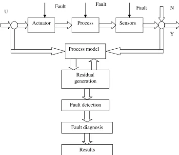
massively in the above references, it is briefly reviewed here for the sake of completion. As shown in figure 1, the diagnostic system contains an actual system and its analytical redundancy that undergoes

the same input. In most cases, the analytical

redundancy is also called a model, which runs in parallel to the actual system. Under healthy conditions, the model output should

be the same as that of the actual system and

Fault Fault _Fault

Actuator Process Sensors

Process model

Residual generation

Fault detection

Fault diagnosis

U N

Y

Results

otherwise the model has to be modified before use. The difference between the model output and the actual system output is called residual. The process to create residual is called residual generation. The

residual is used to detect fault if it occurs in the system. If the residual does not exceed a pre-designed threshold, the system is

referred to as healthy. Once the residual exceeds the threshold, a fault may occur in the system and the diagnostic scheme will send out a fault alarm. This step is called

fault detection. After a fault is detected, fault diagnosis will be applied to allocate and evaluate the fault.

2.2 Basic Theory

Considering a linear control system with

state variable X(t) and output variableY(t),

its model can be represented by state space equations (1) and (2):

) ( ) ( )

(t AX t BU t

X& = + ₍₁₎

) ( )

(t CX t

Y = ₍₂₎

WhereU(t) is input variable, A,B,C are

state matrices with proper dimensions.

A system model can be built up in the form of transfer function, or state observer and even non-parameter model if a parametric model is not available. An observer is used

in this demonstration because it is most frequently used control system modeling. For the system represented by equations (1) and (2), a typical observer gives out its

prediction Xˆ(t) and Yˆ(t) in equations (3)

and (4). )] ( ˆ ) ( [ ) ( ) ( ˆ ) (

ˆ _{t AX t BU t LY t CX t}

X& = + + − ₍₃₎

) ( ˆ ) (

ˆ _{t CX t}

Y = ₍₄₎

Lis the gain matrix of the observer and can be designed according to a specific requirement [17]. A residual ris generated

by calculating the difference between the prediction or observer output and the actual measurement, i.e. ) ( ˆ ) ( ) ( ˆ )

(t Y t Y t CX t Y

r= − = − ₍₅₎

Theoretically, when no fault occurs, _r=0_,

or occurs. However, a real system is always contaminated by disturbance and random noises. Beside, a model that exactly approximates the real system is never achieved. Therefore, a more tolerant

threshold δ _{instead of zero is usually used}

so that the fault detection can be carried out by equation (4).

   

> ≤

δ δ

r r

(6)

2.3 General Methods

From figure 1, students will gain that the

application of the model-based approach consists of the following four steps: modeling, residual generation, fault detecting, and fault diagnosis. In order to

give them a complete knowledge, the general methods involved in these steps are reviewed before an example is given.

Modeling Generally speaking, modeling of a system is to represent a system with mathematical expressions. Transfer function is a simple model of a control system,

especially in SISO system. Some control components have their transfer functions in their specification when in sale. In this case, the transfer function can be taken to represent the system. However, most control

systems are MIMO systems and consist of non-standard components. In this case, state space equations are always used to model

the system provided that all the parameters in the construction of the system can be obtained. Sometimes, a system is so complicated that it is impossible to get its

parameters. A non-parameter model may be developed by using artificial method like neural networks (NN). For simplification, NN method is not included in this demo, and

instead, an example is given to illustrate the conversion of an actual system to a mathematical representation with state space equations.

Residual generation The techniques used to generate residuals differ from method to method. The frequently used methods are Healthy

observer approach, parameter estimation approach, parity space approach and fault detection filter approach. Details of these methods can be found in [4]. Here in this paper, the observer-based approach is used.

Residual is generated by combine the output measurement Y(k) and the observer

estimationYˆ(k).

)) ( ˆ ) ( ( )

(k W Y k Y k

r = − ₍₇₎

Where matrix Wis the weighting matrix.

Fault detection Most fault detection in model-based approach is implemented by comparing the residual signal to the threshold. As mentioned previously, if the

residual doesn’t exceed the threshold, the system is healthy, or otherwise a fault may occur.

There are two types of thresholds, one of which is fixed threshold and the other is

adaptive threshold [4]. The former is simple for design as well as for use. But how to decide the level to be fixed needs to discuss.

The design of threshold is related to the false

alarm rate and the missing alarm rate. The higher the threshold is, the smaller is the false alarm rate but this will decrease the sensitivity to faults and may miss fault alarm. In contrast, if the threshold is

assigned too low, it is more sensitive to faults but there is a risk of false alarm. On the other hand, an adaptive threshold is

designed to adapt to the input. When the model error goes large in its transient period, a relatively large threshold is provided so that a small false alarm rate can be achieved.

For the simplicity, this paper provides a fixed threshold only.

Fault diagnosis Fault diagnosis is to isolate a detected fault, to locate it and sometimes

to indicate the occurring time. Some fault detection methods can locate the fault when it is detected. For example, a parity space will give out the fault as well as its direction.

However, the classifying of the fault needs more complex knowledge. Fuzzy logic and neural network are often used to meet this requirement. This demo does not involve in classification but leaves expendable for this

issue.

3 MODELLING OF THE

EXAMPLE SYSTEM

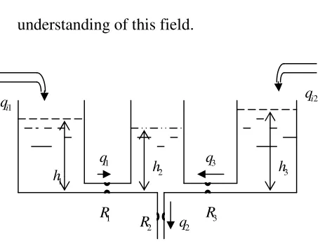
A three-tank system as shown in figure 2 is chosen in this demonstration for the following reasons. It is a realistic physical

representation of many mechanical and chemical processes [18-19], and one which, despite the degree of sophistication to which

control algorithms and model-based approach can be developed, remains sufficiently straight-forward to create within a laboratory. Furthermore, this system is a

non-linear system, which allows us to demonstrate on linearized model and leave students a course work to extend it into non-linear model. Hence, it falls easily within the

realms of desktop demonstration should

anyone wish to develop their own understanding of this field.

3.1 Representation of the System

Figure 2 shows also the operating principle

of the three-tank system. Two inlets on tank

1 and tank 3 supply the flow inputs q_i1and

2

i

q separately. The three tanks are connected

with two pipes with resistances R₁ and R₃to restrict the flow rates q1 and q3 . Liquid (q₂) can only leave through the outlet pipe below tank 2 and encountering

resistanceR₂. The heights h₁, h₂and h₃of the tanks are taken as both state variables and observed variables as well.

1 i

q qi2

1

h h2 h3

1

q q₃

2

q

1

R R₃

2

R

Faults that are simulated in this example are abrupt pulse disturbance in the tanks, blockages in the connection pipes, and tank leakages as well as sensor failures. The demonstration is also open to students to

induce other faults if they like.

3.2 Model in State Sapce Equations

According to the continuous equation and other fluid motion laws [19], the linearized model of it can be given as follows.

1 2 1 1 1 1 1 1 R h h q h dt d S q

q_i − = = _i − − ₍₈₎

3 2 3 2 3 3 3 2 R h h q h dt d S q

q_i − = = _i − − ₍₉₎

2 2 3 2 3 1 2 1 2 2 2 3 1 R h R h h R h h h dt d S q q q − − + − = = − + (10)

Where S_i ( _i=1,2,3 _{) is the cross-section}

areas of the three tanks.

The input variable matrix U is set to be:

T i i T T q q u u

U =[ _{1 2}] =[ _{1 2}] ₍₁₁₎

As mentioned above, both the state variable and the observed output are the liquid levels in the three tanks.

T T T h h h x x x

X =[ _{1 2 3}] =[ _{1 2 3}]

T T T h h h y y y

Y =[ _{1 2 3}] =[ _{1 2 3}]

The model can be represented in the form of

equation (1) and (2) with h dt

d

h&= _{. It is a}

control system with 2 inputs and 3 outputs. The matrices A,B,Care

                  − + + − − = 3 3 3 3 3 2 3 2 1 2 1 2 1 1 1 1 1 1 0 1 ) 1 1 1 ( 1 1 0 1 1 R S R S R S R R R S R S R S R S A (14)                 = 3 1 1 0 0 0 0 1 S S

B (15)

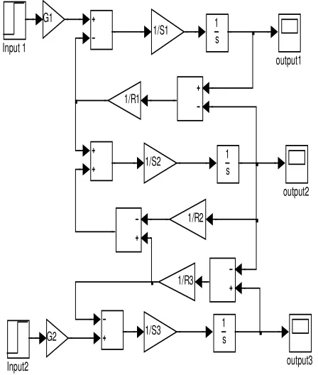
3.3 Model in Simulink

Simulink tool is very powerful platform in system simulation and control [20, 21]. It has the advantages of object and convenient in use. Therefore, it has been widely applied

in many control systems simulation and design. Figure 3 shows the Simulink model of the three-tank system. The inputs are chosen to unit step signal with specific

gains, which can be directly obtained in the

Source Library in Simulink. The parameters in the model are listed in Table 1.

Table 1: The structural parameters of the three-tank system

Parameters S₁(m2) S₂(m2) S₃(m2) Values 7.07e-4 1.3e-3 4.91e-4

Parameters R₁(sec/m2) R₂(sec/m2) R₃(sec/m2) Values 1.724e4 1.e4 2.33e51.e4

4

SIMULATION OF SYSTEM

FAULTS

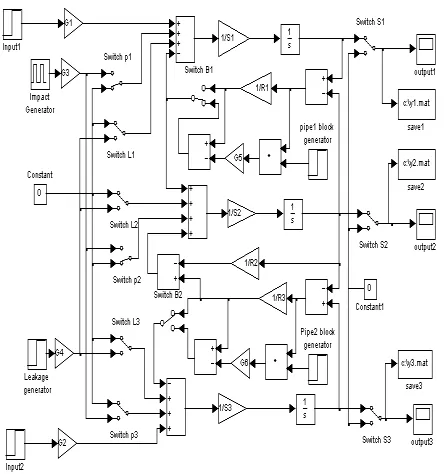
Four types of faults mentioned previously are simulated in the Simulink model. The

first one is an abrupt disturbance fault (ADF). This type of fault can occur in any tank and result in pulses of the liquid level. The second type of fault is a leakage fault

(LF), which may also occur in any of the three tanks and cause the liquid level below the controlled level. The third type of fault is a blockage or partial blockage in the pipes

that connect the tanks, this fault is referred to as a pipe blockage fault (PBF). The fourth

output3 output2 output1

1 s 1 s 1 s

Input2 Input 1

G2 G1

1/R3 1/R2

1/S3 1/S2 1/R1

1/S1

type of fault that can occur is a sensor failure (SF), which will result in false monitoring result. All these faults can be virtually implemented in the Simulink by means of various switches. As shown in

figure 4.

There are 11 switches in figure 4: switches P1 to P3 are for abrupt disturbances, switches L1 to L3 are for leakages, switches

S1 to S3 are for sensor fault and switches B1 and B2 are for pipe blockages. Each switch has two states, one for normal condition

(Off), and the other for faulty condition (On). Table 2 shows the states of these 11 switches and their corresponding faults, “+” and “- ” in table 3.2 refer to states “On” and “Off” respectively. All the 11 switches are

labelled in figure 4. They can be run on their own to implement a single fault or in combination to simulate compound faults. In

addition, some generators like the pulse generator for example are used to induce faults. Changing the gain of a fault input will vary the degree of that fault.

Table 2: Switches and their responding faults

Switches

Tank 1 Tank 2 Tank 3 LF ADF LF ADF LF ADF

P1 - + - - - -

P2 - - - + - -

P3 - - - +

L1 + - - - - -

L2 - - + - - -

L3 - - - - + -

Switches

Pipe blocks

SF1 SF2 SF3 BF1 BF2

B1 + - - - -

B2 - + - - -

S1 - - + - -

S2 - - - + -

S3 - - - - +

Figure 5 shows the simulation results under both normal conditions and faulty

conditions. In all the subplots, the dotted, dashed and solid lines represent the responses of tanks 1, 2 and 3 respectively. Figure 5(a) shows the normal conditions and

Figure 5(b) shows the abrupt disturbance fault (ADF) in tank 1, the ADF is implemented by setting switch P1 to “On” and the others to “Off”. Similarly, Figure

5(c) displays the leakage fault (LF) in tank 3 and Figure 5(d) shows a blockage fault (BF) in pipe one. Figure 5(e) shows a sensor failure in sensor 2 and Figure 5(f) gives the

simulation results for a compound fault. Many other combinations of fault can be simulated by turning on the corresponding switches. It is completely open to students to turn on or off any single switch or any

combination of these 11 switches to check the corresponding results. Results can be displayed on virtual scopes or save to some

Matlab files for further analysis.

5

FAULT DETECTION AND

DIAGNOSIS

Although some changes can be found from the system output as shown in figure 5, it is unclear whether or not these changes are

caused by system faults or by control operations of the system. For example, in figure 5(d) the change may be caused either by a pipe blockage at time instant 40sec or

by an extra system input at time instant 40 sec. A fault diagnosis should be able to distinguish the different sources and remove the influence of the system input. The

advantage of a model-based approach can be Figure 5: Simulation results in fault

demonstrated through the following diagnostic scheme.

5.1 Fault Diagnostic Scheme

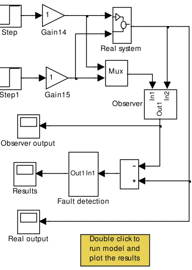
Figure 6 shows a diagnostic schematic in Simulink. A masked Matlab program alongside the diagram will initialize the

parameters and actuate the simulation by double clicking the icon. The “Real system” refers to the three-tank system which is described in figure 4 except that random

noises are added into each output to simulate actual behavior of the three-tank system under fault free and faulty conditions. The “Observer” refers to a full order observer as described by equations (3) to (16) and

parameters in table 1. As shown in figure 7, it shares the same input as the “real system”. The design of gain matrix Lis out of the

scope of this paper and simply set to unit matrix. However, it is changeable for students when they access the masked Matlab program.

A residual generator is designed to compare

the “Observer” outputs and “real system” outputs and to generate the residual signal.

1 Out1

K*u L(y-yhat) 1

s

Integrator K*u

Cx K*u

Bu

K*u

Ax

Add1 Add

2 In2

1 In1

Figure 7: A full order observer

Figure 6: Schematics of fault detection and diagnosis

Double click to run model and plot the results Step1

Step

Results

Real system

Real output Observer output

In

1

In

2

O

u

t1

Observer Mux 1

Gain15 1

Gain14

In1 Out1

Theoretically, any difference between the real measurement and the model prediction can be referred to as a fault. However, it is impossible to develop such an accurate model and model error is inevitable in

practice. Besides, the measurement is often corrupted by noise. In order to cover these error and noise, a threshold is usually

necessary. The fault detection and diagnosis are then carried out with reference to given thresholds including warning levels and fault alarm levels. All response signals and

residual signals are displayed in the scope. Where and when a fault occurred as well as its severity can be established from the scope as shown latter in conjunction with

fault cases.

When running the demonstration, the “Observer” is not altered, whilst the normal and faulty conditions are implemented in the

“Real system”. A graphical representation of the system condition is displayed on the scope. At the same time, the simulation

results are saved into Workspace in Matlab, which allows further analysis to be carried out. The user interface in Simulink is quite convenient to use. For example, it allows other faults to be added to the system or

locations of faults in the system to be changed. These simulation results give details of the system under selected

conditions.

5.2Case Study of Fault Diagnosis

Different types of faults are investigated in this demonstration. The threshold for “fault

level” is set to ±_{1mm and that for “warning}

level” is set to ±_{0.3mm. When the system is}

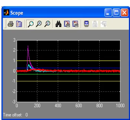
under normal conditions, all three residuals are zeroes or within the warning level thresholds. When a fault occurs in the system, it can be detected on the scope. Figure 8 shows an example of a fault

condition, where the grey line represents the

residual of tank one ( y1 ), the red line represents the residual of tank two (y2) and the green line represents the residual of tank

three ( y3). The same representations will appear in the following figures. In this case, the residual of tank one exceeds the threshold, which means that there is a fault in tank one. The residual response is a pulse

signal, which indicates an abrupt disturbance fault. The fault is detected at time instant 100 sec. Although tank two and three also have abrupt changes in their residuals but

they do not exceed the threshold. This means that both tank two and tank three are affected by the fault in tank one, but no fault occurred in them, except that in tank two the

warning threshold was exceeded. Therefore,

the diagnostic result is that an ADF fault is detected at a time instant 100 sec in tank one.

Figure 9 shows another type of fault, which is detected at a time of 730sec in tank three.

From the residual response of y₃, it is found that the residual exceeds the negative

threshold of warning level at 620sec and then fault level at 730sec. This indicates that a leakage fault (LF) is occurring in tank three.

As mentioned previously, all the signals from the Simulink user interface can be

saved into Workspace in Matlab window for data processing. Figure 10 shows a fault diagnosis carried out in this way. Figure

10(a) displays the same condition as Figure 5(d) with an obvious change in tank one. A false misdiagnosis may be led because only one change can be seen in it. However, with the model-based approach, a residual shown

in Figure 10(b) indicates clearly two different faults occurring in the system. Besides the obvious fault that is detected at

time instant 420sec, there is also an incipient fault present from the beginning. These two faults not only differ in occurring times but also differ in fault types. A leakage fault

exists in tank one, but the pipe blockage fault most likely occurs in the pipe that connects tank one and tank two. This result also demonstrates the significance of a

model-based approach.

Figure 11 shows an example of detection and diagnosis of multiple faults. An ADF is detected at time instant 103sec in tank one,

and then a PBF is detected at time instant 414sec in pipe one. After that, a LF is

0 100 200 300 400 500 600 700 800 900 1000

-5 -4 -3 -2 -1 0 1 2 3 4 5

R

e

s

id

u

a

l

Time

Figure 11: Fault diagnosis of multiple faults

0 100 200 300 400 500 600 700 800 900 1000

-5 0 5 10

S

y

s

te

m

r

e

s

p

o

n

s

e

Time (a)

0 100 200 300 400 500 600 700 800 900 1000

-1 0 1 2

R

e

s

id

u

a

l

Time (b)

detected at time instant 660 sec in tank three.

Sensor faults and many other faults that can be diagnosed with the demonstration are also not addressed here because they only

repeat the procedure with different combinations of switches. They are left for student to play with.

6 CONCLUSIONS

In this paper, the model-based fault detection and diagnosis approach is

implemented on Simulink to provide students with tutorial information of this advance approach. A clear picture of the model-based approach from model

development, data measurement, to residual generation as well as fault detection and diagnosis can be obtained to students by running this demonstration virtually. The

demonstration is made of a multi-tank system, but can be suitable for most of control processes. It shows that the

model-based approach is an advanced method in fault diagnosis of various control systems. The demo works very well and conveniently in computer and no hardware is needed. The cases shown in this paper are only of a small

number. The 11 switches provide for a large amount of different fault combinations, which include component fault, connection

fault and disturbance fault as well as sensor failure. One can view any fault condition just by clicking on and off the correlated switches on the screen.

The demonstration not only answers the question mentioned in introduction, but also provides a transition from theories to applications for model-based approach. In

addition, it provides students an open platform, which allows them to extend the demonstration by either introducing more fault types or using other methods such as

REFERENCES

1 Jones, H. L. (1973). Failure detection in

linear systems, PhD thesis, Dept. of Aeronautics, MIT, Cambridge, Mass. 2 Willsky, A.S. (1976). A survey of design

methods for failure detection systems,

Automatic, Vol. 12, pp601-611.

3 Isermann, R. (1984). Process fault detection based on modeling and

estimation methods – A survey, Automatica, pp387-404.

4 Frank , P. M, Ding, S. X., & Marcu, T. (2000), Model-based fault diagnosis in

technical processes, Tans. of Institute of Measurement and Control, Vol. 22(1), pp57-101.

5 Isermann R. (2005). Model-based fault

detection and diagnosis – status and applications, Annual Review of Control, Vol. 29, pp71-85.

6 Patton R., P. Frank and R. Clark (1989).

Fault diagnosis in dynamic systems, theory and application, Prentice Hall.

7 Chen, J and R. J. Patton (1999). Robust model based fault diagnosis for dynamic systems, Kluwer Academic Publisher, London.

8 Simani, S., Fantuzzi, C., & Patton, R. J.,

(2003). Model-based fault diagnosis in dynamic systems using identification techniques, Springer, London.

9 Patton, R. J. (1997). Robustness in model-based fault diagnosis: The 1995 situation, A Review of Control, Vol. 21, pp. 103-123.

10 Börner, M., Straky, H., Weispfenning, T., & Isermann, R. (2002). Model-based fault detection of vehicle suspension and hydraulic brake systems, Mechatronics,

Vol. 12 pp 999-1010.

11 Patton, R. J. and J. Chen (1991). Robust parity space approach to fault detection based on optimal eign-structure

12 Balle, P. (1999). Fuzzy-model-based parity equations for fault isolation, Control Engineering Practice, Vol. 7, pp. 261-271.

13 Kimmich, F., Schwarte, A., Isermann, R.

(2005). Fault detection for mordern diesel engines using signal-and process model-based methods, Control Enginerering

Practice, Vol. 13, pp189-203.

14 Elshanti, A., Shi Z., & Ball, A. D. (2001). Dispelling the rumours about model-based diagnostics, MARCON’2001,

USA.

15 Isermann, R. (1993). Fault diagnosis of machines via parameter estimation and knowledge processing – tutorial paper,

Automatica, Vol. 29(4), pp 815-835. 16 Isermann R. and P. Balle (1997). Trends

in the application of model-based fault detection and diagnosis of technical

processes, Control Engineering Practice, Vol. 5, pp709-719.

17 Duan, G. (1996). Linear system theory, HIT press, China.

18 Dorf, Richard C., Richard Carl (1998). Modern control systems, 7th edition, Addison-Wesley.

19 J. Schwarzenbch, and K. F. Gill, (1986). System modelling and control, Edward Arnold.

20 Singh, K. K. (2001). System design through Matlab, control toolbox and Simulink, Springer, London.

21 Huning-huei Su, et al, (2002). Learning