Improved Gaussian Filtering Model for Highly Noised Image by Salt and Pepper

2017 2nd _{International Conference on Computer Science and Technology (CST 2017)}

ISBN: 978-1-60595-461-5

Improved Gaussian Filtering Model for Highly

Noised Image by Salt and Pepper

Mansoor Ahmed Khuhro

_{*, Dong-jun HUANG}

_{, Shao-nian}

HUANG

_{and Li-li YANG}

1_{School of Information Science and Engineering, Central South University,}

Changsha, Hunan PRC China, 410083

2_{School of Computer and Information Engineering, Hunan University of Commerce,}

Changsha, Hunan PRC China, 420005

a_{[email protected]}

*Corresponding author

Keywords: Noise detection, Salt & pepper noise, neighborhood pixels, Median Filter, Gaussian Filter.

Abstract. Image denoising is one of the most significant areas within digital image processing. Such as impulse noise can appear in images during acquisition, storage, or transmission which can latterly affect stage of processing image, and may not remove properly during preserving the details of effected image. After reviewing the different techniques, in this paper, we have proposed a significant algorithm which does detect and reduce the level of salt and pepper noise in less computation time and techniques.

Introduction

Vision is the most advanced in our consciousness, it is not surprising that the images are playing the most important role in our perception. Typically, digital videos are damaged by unwanted random differences in the values of topics that are known as noise. The existence of noise is caused by a faulty image sensor, channel noise through image transmissions and video sequences. However, an exemplary embodiment of a visual band is limited to the electromagnetic (EM) spectrum in the entire electromagnetic spectrum from gamma to radio waves. Which can operate on images that humans are not accustomed to the source associated with the image.

Devices and applications of computer produced driven by the innovation in technology have rearranged the operation which consists of images those involved more relevant ideas about these issues [1]. Past decades many researchers have been directed to multiple directions for profiting from the techniques of image processing in our daily life. Medical imaging is a valuable tool in medicine. In various medical imaging techniques, such as CT, US and X-ray, magnetic resonance imaging (MRI) [2] provides more efficient information about the anatomical structure of the medical images.

Background

preserving the details. This problem rises in many fields such as medical imaging [3], and the analysis of satellite images, there are different types of noise models which include thermal noise, RF noise, Gaussian noise, salt and pepper noise, speckle noise and Brownian noise [1,4].

The widespread sort of noise is impulse noise [5], which is known as salt and pepper. This type of noise randomly changes intensities of a number of pixels to the max or min value of the intensity range on the image [6].

A number of filter methods have been recommended for reducing the noises from images that are simultaneously corrupted by impulse noise and so they are the best methods to reduce noise because they are easy put to practice on hardware.

The filters which are usually designed for the removal of noise from images [7] are categorized into different types considering several particular functions. Although liner filters [8] degrade the edges of images, it can conveniently have used in the removal Gaussian noise as well as it also performs good impulse noise.

Nonlinear method fails to exclusively apply the inverse approach [9,10]. It’s using an iterative method to generate the successive perfection to the renewal pixels until it reaches to the end condition. Somehow it is manageable with certain lost frequency factors with non-Gaussian noise.

Filtering the salt and pepper noise MF is one of the most common method [10]. This method is non-linear and this fact that it does not damage the edge details of image which makes it as reliable filter [12]. The main concept is to analyze a sample model of the input determine the value of a special pixel according to neighboring pixels. The execution utilizing a window containing an odd number of the model [13-14]. The values in the window are fixed into numerical order; the median value to model in the center of the window is picked as the output. Which is Convenient to execute and also efficient. Although it has a primary drawback to working only on low densities. Whenever density level is higher over 50% then the edge particulars of the original image is not sustained.

Neighbors Pixels

A pixel at coordinates ( , ) has four horizontal and vertical neighbors whose coordinates are given by below equation:

( + 1, ), ( − 1, ), ( , + 1), ( , − 1)

And for four diagonal neighbors of have coordinates

( + 1, + 1), ( + 1, − 1), ( − 1, + 1), ( − 1, − 1)

And are denoted by ( ). These points, together with the 4-neighors, are called the

8 − ℎ of , denoted ( ). As before some of the neighbor locations in ( )

and ( ) fall outside the image if ( , ) is on the border of the image. Denoising image at the pixel ( , ), where the neighbor pixel size is 3x3.

If − > 0, then the median value is /( , ). If /( , ) < ( , ), then /( , )

is noise.

Gaussian Filter

kernel and then summing to result in the output array. The Gaussian filter performs support in 8-bit or 32-bit floating point formats, and it can don't in place For the Gaussian blur the initially two parameters give the width and height of the filter window; the (optional) third parameter indicates the sigma value (half width at half max) of the Gaussian kernel. In case the third parameter is not specified, then the Gaussian will probably be automatically identified from the window size using the following equation:

=

2 − 1 0.30 + 0.80, = 1

=

2 − 1 0.30 + 0.80, = 2

Gaussian smoothing constructs a weighted mean of every pixel as well as their neighboring elements. The weighting carries two elements, the first in which there is a similar weighting utilized by Gaussian smoothing. The second element is as well as Gaussian weighting however located not on the spatial range from the central pixel. Gaussian noise has a Gaussian distribution which has bell shaped probability distribution function given by:

( , ) = 1

√2 =

1 √2

1 √2

The 2 Gaussian can be express as the product of tow function. One a function of and the other is a function of .

( ) = 1

√2

( ) /

Where the represents the gray level of image and indicates the mean function, as well as is the standard deviation of the noise.

Here if we computer the noise using Gaussian filters at different scales, the different values are obtained. Looking at the evolution of filter response for the different scale factors, we obtain the curve which eventually reaches at the maximum value at value. The scale variant features should be detected as local maximum in spatial space in the image.

Algorithm: Gaussian White noise

Input: Img1. The image to be modified (by adding white noise) Mean:

Sigma:

Output: The noised Image

BEGIN

NoiesArray = Img.Copy() Fill.NoiseArray()

For each v Value of NoiseArray

RandomPixel(Img1) = v + 255 //White Color Next

Salt and Pepper Noise

This color improvement simply signifies the name of noise. White color indicates the value 255 and it is called as salt noise while black color indicates the value 0 and it is known as pepper noise. Impulse noise can occur in image negatively or positively. Impulse corruption usually is large compared with the strength of the image signal, impulse noise normally is digitalized as high value in an image. So, therefore, the assumption is generally that a and b are overloaded value in the sense that they are similar to the max and min allowed values in the digital image. The probability density function in impulse noise is generated by the below given formula.

( ) = ==

0 ℎ

When > , brightness of will appear as a light dot in image. In opposition, level will appear just like a dark dot. If either or is zero.

Algorithm: Add Salt & Paper in Image Input: Img1-> Original Image

n -> The level of distorting image

Output: Img2 -> The image modified, including salt and paper Begin

For k = 0 to n

Rand = Get_RandomValue()

ImgColors = Get_ImageColors(Img1) ImgRows = Get_ImageRows(Img1) I = Rand % ImgColors

if Image_Pixel(Img1) is GrayLevel

Img1[ImgRows, ImgColors] = WhiteColor Else If Image_Pixel(Img1) is GrayLevel

Img1[ImgRows, ImgColors].Red = WhiteColor Img1[ImgRows, ImgColors].Green = WhiteColor Img1[ImgRows, ImgColors].Blue = WhiteColor End For

Img2 = Img1 Return Img2

Conversation Color to Gray Image

The purpose how come grayscale representations tend to be chosen for taking out descriptors rather than operational on color images straight is that grayscale simplifies the algorithm as well as minimizes computational requirements. In fact, the color might be of limited advantage in numerous applications and including unnecessary information could increase the volume of training data supposed to achieve good performance.

RGB A to GRAY: Y ← 0.299 ∙ R + 0.587 ∙ G + 0.114 ∙ B

Algorithm: Reduce Color

Input: Img1 Image to be reduce the color div: Given number

BEGIN

For Each r Rows of Image

For Each c Columns of Image //scan every pixel

CurrentPixel = CurrentPixel.Value / div * div + div/2 //Get the neighbor pixel average color

Next Column Next Row

END

Experimental Results.

In this paper, the algorithm is verified on different color images. We have implemented our algorithm using OpenCV 3.1 and VS 2013, the Operating environment is windows10, and the memory of the system used is 6 GB. The images are corrupted by fixed value impulse salt and pepper noise, performance is quantitatively measured with various noise densities for Peak-signal-to-Noise and Mean Square Error(MSE).

= 10 (255)

= ∑ ∑ ( , ) − ( , )

Here m x n is the size of the image. ( , ) represents the original image and ( , )

represents de-noised image and 1 (i, j) represents noisy image. The noise density is varied from 10% to 90%. The results show improved performance.

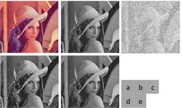
Figure 2: (a) Shows Original Image (b) Conversation from color to Gray

(c) Salt & pepper 90% (d) effect after Median filter (d) Reconstruction of image with proposed method.

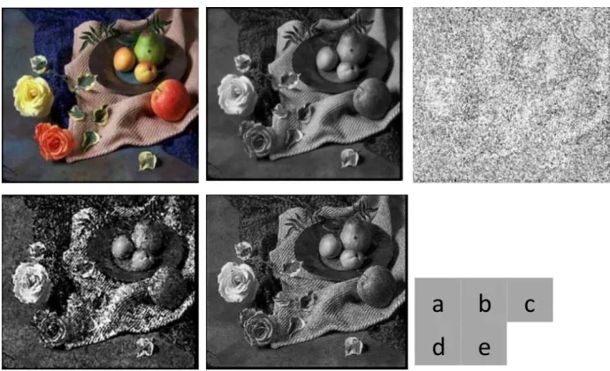
Figure 3: (a) Shows Original Image (b) Conversation from color to Gray (c) Salt & pepper 90% (d) effect after Median filter (e) Reconstruction of image with proposed method.

Conclusion

In this paper, we have proposed an algorithm to overturn salt and pepper noise from different corrupted image type such as jpg, bmp etc. at different level. It offers a satisfactory reinstatement of images at higher noise level when many other median filters produce the recovered images are difficult to identify. The visual features and quantitative results obviously, state that the proposed filter functions far better than currently recommended filter methods concerning impulse noise removal and details efficiency.

At the same time, we believe that the suggested method is exposed to be advanced in serval ways including implementation and smoothness of an image, and application to further noise types at present can be efficiently employed on the salt and pepper noise condition.

Acknowledgment

This work was supported by the Project of National Science Fund of China (NO .60873188)

References

[1] A. K. Saini, H. S. Bhadauria, and A. Singh. “A Survey of Noise Removal Methodologies for Lung Cancer Diagnosis,” 2016 Second Int. Conf. Comput. Intell. Commun. Technol., pp. 673–678, 2016.

[2] M. G. Sumithra, and B. Deepa. “Performance Analysis of Various Segmentation Techniques for Detection of Brain Abnormality,” pp. 2058–2063, 2016.

[3] S. Vb, and G Raju. “Literature Review of fMRI Image Processing Techniques,” pp. 1473–1476, 2016.

[4] H. Gómez-moreno, P. Gil-jiménez, S. Lafuente-arroyo, R. López-sastre, and S. Maldonado-bascón. “A ‘Salt and Pepper’ Noise Reduction Scheme for Digital Images Based on Support Vector Machines Classification and Regression,” vol. 2014, 2014. [5] H. Al-Khaffaf, a Z. Talib, and R. a Salam. “Removing salt-and-pepper noise from binary images of engineering drawings,” 2008 19th Int. Conf. Pattern Recognit., pp. 1–4, 2008.

[6] W. Li, Y. Sun, and S. Chen. “A new algorithm for removal of high-density salt and pepper noises,” Proc. 2009 2nd Int. Congr. Image Signal Process. CISP’09, pp. 0–3, 2009.

[7] V. R. V. Kumar, and G. Nanalya. “Removal of Salt and Pepper Noise Using Robust M-Filter,” no. 978, pp. 175–178, 2016.

[8] O. Rioul. “A spectral algorithm for removing salt and pepper from images,” IEEE Digit. Signal Process. Work., pp. 275–278, 1996.

[9] S. Feizi, S. Zahedpour, M. Soltanolkotabi, A. Amini, and F. Marvasti. “Salt and pepper noise removal for image signals,” 2008 Int. Conf. Telecommun. ICT, 2008.

[10] L. Shao. “Up-scaling images in presence of salt and pepper noise,” ELECTRONICS LETTERS 5th July 2007 Vol. 43 No. 14.

[12] Y. Wei, S. Yan, L. Yang, and Y. Fu. “An improved median filter for removing extensive salt and pepper noise,” Proc. - 2014 Int. Conf. Mechatronics Control. ICMC 2014, no.

[13] G. Xu and Y. Lin. “An Efficient Restoration Algorithm for Images Corrupted with Salt and Pepper Noise,” pp. 184–188, 2016.