A comparison of Value at Risk methods in portfolios with linear and non linear financial instruments

(1)

(2)

2

Research Methodology

Evaluation of research philosophies and perspectives. Justification of

methodological approach, sampling strategy, data analysis and reliability and validity measures as applicable

Supervisor Comments:

15% 2nd_{marker Comments:}

Data Analysis and Interpretation Evidence of rigor in data analysis and interpretation procedures, identification of key patterns and themes in the research data, integration of academic theory into explanation of findings

(3)

3

Conclusions and Recommendations

Research question and objectives addressed with implications to theoretical and managerial concepts considered. Recommendations provided for theory, practice and future research

10% 2nd_{marker Comments:}

Organisation, presentation and references.

Well structured and ordered dissertation with correct use of grammar and syntax. In-text citation and bibliography

conforming to “Cite Them Right”

(4)

4

Total

First Marker Total

100%

Second Marker Total

Supervisor General Comments: Agreed Mark:

2nd_{Marker General Comments:}

Supervisor’s Name: ……….. Signature: ………

(5)

5

A comparison of Value at Risk methods in portfolios with linear and non-linear financial instruments

A dissertation submitted in partial fulfilment of the requirements of the School of Business and Law, University of East London for the degree of Finance and Risk MSc

September 2016

Word count: 13,114

I declare that no material contained in the thesis has been used in any other submission for an academic award

(6)

6

Dissertation Deposit Agreement

Libraries and Learning Services at UEL is compiling a collection of dissertations identified by academic staff as being of high quality. These dissertations will be included on ROAR the UEL Institutional Repository as examples for other students following the same courses in the future, and as a showcase of the best student work produced at UEL.

This Agreement details the permission we seek from you as the author to make your dissertation available. It allows UEL to add it to ROAR and make it available to others. You can choose whether you only want the dissertation seen by other students and staff at UEL (“Closed Access”) or by everyone worldwide (“Open Access”).

I DECLARE AS FOLLOWS:

 That I am the author and owner of the copyright in the Work and grant the University of East London a licence to make available the Work in digitised format through the Institutional Repository for the purposes of non-commercial research, private study, criticism, review and news reporting, illustration for teaching, and/or other educational purposes in electronic or print form

 That if my dissertation does include any substantial subsidiary material owned by third-party copyright holders, I have sought and obtained permission to include it in any version of my Work available in digital format via a stand-alone device or a communications network and that this permission encompasses the rights that I have granted to the University of East London.

 That I grant a non-exclusive licence to the University of East London and the user of the Work through this agreement. I retain all rights in the Work including my moral right to be identified as the author.

 That I agree for a relevant academic to nominate my Work for adding to ROAR if it meets their criteria for inclusion, but understand that only a few dissertations are selected.

 That if the repository administrators encounter problems with any digital file I supply, the administrators may change the format of the file. I also agree that the Institutional Repository administrators may, without changing content, migrate the Work to any medium or format for the purpose of future preservation and accessibility.

 That I have exercised reasonable care to ensure that the Work is original, and does not to the best of my knowledge break any UK law, infringe any third party's copyright or other Intellectual Property Right, or contain any confidential material.

 That I understand that the University of East London does not have any obligation to take legal action on behalf of myself, or other rights holders, in the event of infringement of intellectual property rights, breach of contract or of any other right, in the Work.

I FURTHER DECLARE:

 That I can choose to declare my Work “Open Access”, available to anyone worldwide using ROAR without barriers and that files will also be available to automated agents, and may be searched and copied by text mining and plagiarism detection software.  That if I do not choose the Open Access option, the Work will only be available for use

(7)

7 X

/cont Dissertation Details

Field Name Details to complete

Title of thesis

Full title, including any subtitle

“A comparison of Value at Risk methods in portfolios with linear and non-linear financial instruments”

Supervisor(s)/advisor

Separate the surname (family name) from the forenames, given names or initials with a comma, e.g. Smith, Andrew J.

Tat Chan

Author Affiliation

Name of school where you were based

School of Business and Law

Qualification name

E.g. MA, MSc, MRes, PGDip

MSc

Course Title

The title of the course e.g.

Finance and Risk

Date of Dissertation

Date submitted in format: YYYY-MM

2016-09

Does your dissertation contain primary research data? (If the answer to this question is yes, please make sure to include your Research Ethics application as an appendices to your dissertation)

Yes No

Do you want to make the dissertation Open Access (on the public web) or Closed Access (for UEL users only)?

Open Closed

By returning this form electronically from a recognised UEL email address or UEL network system, I grant UEL the deposit agreement detailed above. I understand inclusion on and removal from ROAR is at UEL’s discretion.

Student Number:1444031 Date: 10/09/2016

(8)

8

A comparison of Value at Risk methods in

portfolios with linear and non-linear

financial instruments

Daniela Martins Neto

University of East London

(9)

9

Abstract

This paper intends to critically evaluate and compare the most used Value at Risk (VaR) methods, whilst also presenting the strengths and weaknesses of each model. The analysis is based on a stock (linear) portfolio and an option (non-linear) portfolio. The methodologies applied are the delta-normal, delta gamma, historical simulation and Monte Carlo simulation, computed to one and five days time horizon with 95% and 99% of confidence level.

The results demonstrate that Monte Carlo simulation provided the most accurate risk measure and consistent results for both portfolios which reinforce the flexibility of the model to estimate VaR. Although the Delta Gamma also showed an accurate VaR for the option portfolio, it is complex and demands a high level of calculation which can become complicated and costly. The historical simulation for both portfolios were overestimated because of the fact that the historical simulation is strongly based on historical data. Additionally, the delta normal was shown to be a weak model as it does not properly present accuracy even for the linear portfolio. This is because this model is heavily based on normal distributions, and in practice fat tails are more frequent than predicted by the model.

The benefit of portfolio diversification in the VaR measure was also proved in this paper. It presented a substantial improvement in the VaR measure when considering in the calculations the correlation between instruments. Once more, the Monte Carlo simulation presented a higher efficiency in VaR measures with the diversified portfolio.

(10)

10

The last global economic disasters led to the bankruptcies of large and robust financial institutions that in many cases were considered systemically key for the industry. The interconnection between these financial institutions allowed an increase in the size of the disasters in the market. Most crises were caused as a result of a failure of risk management systems. The 2007-2008 crisis highlighted serious deficiencies in risk management and demonstrated the importance of an efficient risk management process (Jorion, 2009). Thus, the weaknesses of the world regulatory system were exposed and criticised by the financial market which raised the necessity of a more rigorous international regulation to control and monitor the financial market. As a consequence, the financial regulation was reformed and new measurements and controls were established, for instance, the Dodd-Frank Act and the Systemically Important Financial Institution – SIFI regulation.

In order to adhere to international agreements defined by the regulators, financial institutions had to develop tools and systems to measure and control their risk exposure. Using statistical and mathematical approaches to measure risk, JP Morgan developed the RiskMetrics which was published in 1994 through a technical document available for all market participants. It increased the popularity of the Value at Risk – VaR methodology that became a reference in estimating market risk. As a result, other financial institutions started developing improvements and variants of the VaR.

VaR reflects the maximum expected loss an institution can obtain given a time horizon and confidence level. It is widely used by banks and financial regulators as a standard measure to monitor and compare risks in different sectors. The VaR popularity is a result of a combination of factors. Firstly, the improvement of the banking regulation on risk management such as the Basel Accord. Secondly, the globalisation of the financial market that increases volatility and exposure to several risks. Lastly, the technology which enhances the risk control (Jorion, 2007). With regards to managing and supervising risk exposure, banks and regulators are able to assess the likely loss of a portfolio through the VaR.

(12)

12 On the last BCBS (Basel Committee on Banking Supervision) standard publication about capital requirement for market risk, it is recommended the VaR application for measuring market and default risks (BCBS, 2016). There are also other BCBS’s publications suggesting VAR methodology to compute different types of risk exposures. Additionally, BCBS constantly issues guidelines about capital requirement which might be followed by central banks and financial institutions as best practices. For this reason, the decision of what model should be used for risk measurement becomes crucial for all banks and financial institutions. This is because, besides managing risks prudently, banks need to be in compliance with regulation in terms of holding capital according to their risk measured. Cuoco and Liu (2005) suggest VaR as an efficient methodology to estimate risk for capital allocation, they also find that it can contribute to reveal this risks. All financial institutions aim to be efficient in managing risk. In order to achieve it, they invest effort in choosing an adequate VaR methodology among the numerous approaches available. Moreover, they can create their own proprietary model that often better fits their portfolios, risk exposures and capital requirements. These internal models usually are based on VaR methodology.

Due to the importance of the VaR as a risk measure recommended by regulation and its widespread reach all over the international market, an important question arises: which VaR method is able to deliver the most accurate risk exposure estimation? The theory says that there is no single winner and that it depends on the portfolio composition and strategy. Lambadrais et al (2000) present a comparison between Monte Carlo and historical simulations for linear and non-linear portfolios, and conclude that the Monte Carlo simulation shows more accurate performances in the linear portfolio; however, for the non-linear portfolio any model performs well. Chapter 2, the literature review, is illustrated with more papers that compare different VaR methodologies.

(13)

13

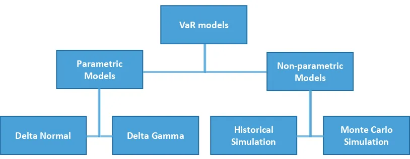
[image:13.595.120.527.101.259.2]

Figure 1 – Different VaR methodologies

This work is organised as follows. The next section, chapter 2, presents a review of the traditional and

more recent literature related to VaR. Chapter 3 describes the main VaR methodologies which are used

later to evaluate the portfolio’s market risk. In chapter 4, a comparison of four VaR methods is made

by applying them to a linear stock portfolio and a non-linear option portfolio, also the advantages and

weaknesses of each model are presented. Chapter 5 suggests an alternative VaR approach based on

extreme values. Chapter 6 presents the general conclusion. Finally, chapter 7 suggests the

recommendations.

2. Critical Literature Review

One of the most robust pieces of research about the VaR methods emanates from Duffie and Pan

(1997). They compare the delta gamma method with the Monte Carlo simulation for an option portfolio

randomly selected. It is composed of 10,996 options with 418 different underlying ones exposed by

different risk factors: commodities, equity, fixed income and foreign exchange. This study uses some

identical parameters applied in the RiskMetrics (1996), such as standard deviation. This research finds

that the Monte Carlo simulation, with a stochastic process and a lognormal distribution of the returns,

presents higher VaR than the delta gamma model. This is based on a 99% confidence level, and also

considering long and short positions. This difference between the approaches is 0.1% of the portfolio

value for 1 day VaR and 1.8% for 10 days VaR. This is due to the normality (fat tails) and

non-linearity of the options.

A highly significant contribution to spreading the VaR methodology is the RiskMetrics (1996) by JP

Morgan and Reuters. This technical document provides enhancement in the parameters estimation to

calculate the VaR analytically for a portfolio. The assumptions used makes the VaR application simpler Historical

Simulation

VaR models

Non-parametric Models

Monte Carlo Simulation

Delta Gamma

Delta Normal

(14)

14 and available for any financial institution. Regarding the distributions, this study assumes that the standardised returns have a conditional normal distribution although they might not be normal because, in practice, fat tails are common. The standardised returns are estimated as the return divided by the standard deviation. The research’s attention to this standardised returns allows seeing the importance of the proportion of the return associated with standard deviation. So, a high profit or loss due to a great volatility might lead to a low standardised return while a great return in a low volatile scenario, might result in a high standardised return. The assumption of the standardised returns allows increase the possibility of outliers in the distribution increasing more than what could exist in a normal distribution. In this way the RiskMetrics can be applied to normal mixture distributions that enables the inclusion of larger probability for outliers. However, in this approach what is needed is to estimate the probability of the jumps and their standard deviations, which is neither simple nor effortless as they are rare.

RiskMetrics (1996) also explains some fundamental procedures in the VaR system. Firstly, it presents three necessary parameters to estimate the VaR: the time horizon, the confidence level and the currency used to measure risk. Then, it shows the importance of identifying the cash flow and Marked to Market (MtM) of the portfolio positions, and applying the mapping process where the positions are aggregated in risk factors. Therefore, this paper demonstrates that a crucial step is to choose the method to estimate the VaR. If it is expected that the portfolio will have an approximated normal condition, the RiskMetrics approach (delta normal) should be applied. On the other hand, if the portfolio is exposed to non-linearity and the assumption of normality is not expected, two methodologies should be chosen: the delta gamma and Monte Carlo.

Additionally, Hull and White (1998) recommend alternatives to measuring VaR when the observations are not normally distributed. It enables the calculation of any probability distribution for these observations, but the distribution still has to be a multivariate normal distribution. There are also other studies that create relevant variations of the distribution, however they might lead with some issues. Assessing inputs for non-normal methods is likely to be hard, mainly when using historical data. Also, it is gradually harder to measure losses with asymmetric and fat tailed distribution than with normal distributions.

(15)

15 the returns does not change during the given time. This is the homoscedasticity process. On the other hand, according to Engle (2001), more accurate VaR calculation can be realised when considering possible changes in the standard deviation over time. Using this approach, he argues for the autoregressive conditional heteroscedasticity (ARCH) and the generalised autoregressive conditional heteroscedasticity (GARCH) to deal with standard deviation and variance more precisely. However, the disadvantage of applying these techniques to calculate the variance and covariance of the VaR is that it is only used in portfolios with linear market risk exposure not including options.

Regarding to accuracy and computational time, Pritsker (1997) analyses and compares six VaR models for non-linear instruments and 500 random portfolios. The instruments are call and put options classified in long and short positions, in/out the money and different maturities. The portfolios comprehend underlying options. The results show that 25% of the 500 portfolios under/overestimate the VaR by 10%. When the underlying options of the portfolios are deep out the money or with a short time to expiration the estimations are weaker. For the call options, alternatives models of the delta normal and delta gamma are also applied and the results are highly overestimated. For the put options, the VaR models are underestimated. In terms of the trade-off between accuracy and time consumption, the delta gamma Monte Carlo presents the best performance. Moreover, Krause and Paolella (2014) present a VaR approach based on GARCH for return distributions that contain leptokurtosis, asymmetry and conditional heteroscedasticity. This paper illustrates that this approach works properly and deliver higher results than traditional methods. This is achievable due to the use of quicker and simpler ways to get the risk measure. Also, this work calculates the VaR using samples of 250 observations or less.

Moreover, Castellacci and Siclari (2003) measure VaR methods using 5 approaches for non-linear instruments (option strategies) modelling the return distribution as multi normal random observations. The models applied are: full Monte Carlo, delta gamma Monte Carlo, delta normal, delta gamma normal and Cornish Fisher. Although the theory suggests the delta gamma approach for option portfolios, this paper presents a better performance in the delta normal VaR measure. However, it shows relevant improvements in the delta gamma approach instead of Monte Carlo as it considers the gammas. This is a result of the non-diagonal function in the gamma matrix, also the effect of correlation between the instrument of the portfolios. The delta gamma Monte Carlo approach shows a good performance with moderate computational time. Broadly speaking, this paper demonstrates that the parametric models overestimate the VaR while delta gamma Monte Carlo slightly underestimates the VaR.

(16)

16 model and the historical simulation. He uses 1000 portfolios randomly selected which are exposed to foreign exchange. The application of 9 methods to measure the VaR is done by comparing the real loss with its estimate. Finally, he does not recommend any method. He argues that extreme values are more frequent than assumed by the normal distribution and the volatility is not constant over time.

Additionally, Lambadrais et al (2000) compare VaR methods applying Monte Carlo and historical simulations in the Greek bond and stock markets. For the two methods, portfolios with linear and non-linear instruments are applied. The findings are different for non-linear and non-non-linear portfolios. For the linear portfolio, the Monte Carlo simulation performs well but in the historical simulation the VaR is overestimated. For the non-linear portfolio, both methods do not demonstrate clear results as their numbers differ in the measurement test. The paper also shows that for linear portfolios, the accuracy of the models depends on the confidence level. Emmer et al (2015) compare VaR among other approaches to estimate market risk. This analysis finds positive and negative aspects of VaR. The negative point is that VaR does not account for tail risks beyond the VaR which can be worse when leading with risks that have different tails. In terms of robustness, they argue that VaR has superior results.

Kuester et al. (2006) also compare different VaR models applying more than 30 years of daily price for a stock index portfolio. This paper’s results show that despite most models being accepted by the regulator, they are not satisfactory. The most accurate results are from a GARCH hybrid model with Extreme Value Theory, a variant of a filtered historical simulation and a heteroskedastic mixture distribution. The model shows that for the parametric approaches a significant result in violation frequency is likely to be seen when considering scale dynamics, and also, when considering heteroskedastic, it results in unclustered VaR violations. This paper demonstrates that normality is reached with innovation distribution that includes skewness and fat tails.

(17)

17 Reuse (2010) compares the traditional delta normal VaR method with more modern VaR method such as the historical simulation with copula functions, during a financial crisis scenario using 10 years data. Surprisingly, his results show that the crisis has no effect in the portfolio optimization but the VaR methods present considerable different estimates even more when increasing time horizon. The ideas he presents behind the results is that while in the historical simulations risk is captured by the difference between expected loss and historical data; in the delta normal, risk is captured by the expected loss and the current value, also, in the delta normal, there is a linear approximation which not necessarily illustrate the real data. Regarding the portfolio selection, he argues that the historical simulation gives a better combination of assets, and the delta normal method increases risk exposure. Consequently, the diversification factor is more efficient in the historical simulation. Additionally, the results do not change when raising confidence level. However, this paper shows that the weaknesses in both models is being dependent on historical data, and that is difficult to define the period accurately to have a precise VaR estimation. He also argument that VaR models should be less complicated to understand and apply by the risk managers; it sometimes is more important than accuracy.

According to Trenca et al. (2011), the portfolio characteristics are very important factor to consider when selecting which VaR model to use. This work captures parametric (delta normal) and non-parametric models (historical simulation, filtered historical simulation - FHS and Monte Carlo), also it deals with volatility and correlation calculations (GARCH model). They argue that even though the delta normal is the simplest to apply, it usually underestimates the VaR and capital allocation as it does not take account the fat tails that, in practice, is quite common. They reinforce that VaR is one of the most popular approach to control, measure and that it can prevent market risk as well.

(18)

18 Regarding the historical simulation approaches, Cabedo and Moya (2003) develop a VaR method called historical simulation with ARMA (autoregressive moving average model) forecast - HSAF. This model does not use a simple time series of historical prices but rather the distribution of forecasting errors. In order to measure VaR, this model captures the autocorrelation of the historical prices and, estimates the historical return in absolute values, applying the autocorrelation functions to forecast precisely the future returns. Using oil prices, the researchers compare their own model with the other two VaR methodologies: the standard historical simulation and the delta normal method. The results show a better performance in the HSAF model rather than in the two traditional models. A positive aspect of the HSAF is that it does not need statistical assumption in the distribution of the historical prices as in the ARCH and GARCH approaches. However, if the distribution of returns is stationary or non-statistically significant, the VaR calculation of HSAF is the same as the standard historical simulation.

Additionally, Boudoukh et al. (1998) investigate the limitations of the variants in historical simulations. They develop a hybrid approach combining the RiskMetricks and the historical simulation to improve the VaR for fat tailed distributions. This approach consists of calculating the percentile of the return distribution by declining weights in the historical data through a decay factor. As the data is more recent, it has more weight in the analysis. This model is applied to a stock portfolio with historical data of 250 days including equally the period before and after the stock market crash of 19th_{October 1987.}

The results demonstrate that the VaR using the hybrid approach for this portfolio is not over/underestimated even on the day after the crash because the days are equally weighted according to the model. As the recent past has more weight in the data, is does not cause an outlier in the return distribution.

In a different way but with the same aim of updating historical data, Hull and White (1998) propose improvements in historical VaR by adjusting the data to include changes in volatility over the time. For instance, they argue that when using series with different volatilities during the time, if the series are updated before calculating the VaR, it can improve the risk measure. Using GARCH and exponentially weighted moving average models, the simulation is applied to 9 years of historical data, 12 different exchange rates and 5 stock indices and shows relevant results in estimating the VaR.

(19)

19 time-varying correlations and to select an adequate length of the past sample. Also, previous tests illustrate that applying the FHS for 2 years of daily returns a 99% confidence level and 10 days of time horizon, might not have sufficient outliers to estimate the VaR precisely.

Regarding to the Monte Carlo approach, the greatest weakness of the Monte Carlo simulation is computational time as the model requires plenty of random scenarios to compute the VaR. Jamshidian and Zhu (1997) suggest a scenario simulation approach for the Monte Carlo VaR for large portfolios with exposure to multi market risks. This method applies a limited and manageable quantity of scenarios instead of multivariate distribution of returns. This method also can be used in credit risks. The findings show a large computational efficiency to estimate VaR precisely for portfolios highly exposed to risk factors. Moreover, Frye (1997) presents a method to reduce the quantity of random scenarios by pre-selecting and computing shocks in the data analysis.

Furthermore, Glasserman et al. (2000) propose a model to simplify the sampling of scenarios in Monte Carlo simulation by using the delta-gamma approach. As deltas and gammas are used in valuations and other analyses, they are often accessible without further effort. The results show that this model decreases the quantity of simulations to achieve accuracy, and that consequently it is more efficient in terms of computational time and cost to generate the Monte Carlo VaR. Additionally, Botev et al. (2010) suggest a new Monte Carlo model through generalised splitting algorithm which they say provides superior results regards to accuracy and time consumption.

Despite being the most widespread methodology to measure risk, there is relevant research that does not recommend VaR. Beder (1995) argues that VaR is highly seductive but dangerous as a method to estimate risk. After applying 8 methods for 3 portfolios, this work finds significant inaccuracies in the VaR estimations. Also, it points out that VaR is heavily dependent on parameters, data and assumptions and concludes that VaR is not a sufficient tool to control risk. Other papers show that it is totally possible to find different outputs from the same portfolio and underlying asset considering the same approach. Berkowitz, O’Brien (2002), Ju and Pearson (1998) argue that the VaR estimation for some banks are highly imprecise. Artzner et al (1997) also criticise VaR. They mention examples where a portfolio is divided into 2 sub-portfolios and the calculation of their VaR demonstrates that the sum of the VaR of the 2 sub-portfolios is lower that the VaR of the portfolio before being divided. It should account for the correlation of the instruments that compose the portfolio. This would be an issue for VaR limits in individual books. Also Artzner et al (1997) say that VaR fails in neglecting the size of the loss that exceeds it.

(20)

20 and foreign exchange rates in a stressed scenario. They also discuss the issues can be caused by this risk and make a comparison between VaR and an alternative risk measure, known as Expected Shortfall. Their findings show that this alternative in many cases can properly replace VaR; however, it needs more sample size to result a precise measure.

Similar to any other mathematical or statistical method, VaR can fail if its assumptions or parameters are not precise. Alexander and Sarabia (2012) present a model to deal with the problem of imprecise VaR due to the inadequate choice of the VaR approach or inaccurate VaR parameter calculations. They say this model provides a key to avoid model risk and to attend the capital regulation that requires institutions to control it. This is based on a comparison between a benchmark VaR and the daily VaR computed by the institution. They argue that the benchmark VaR should consider the total information, beliefs and the maximum possible distribution. It should also be determined by the local regulator and applied for institutions. The difference in the quantile between the VaR and its benchmark would determine the model risk and it should be adjusted in the capital requirement. They also illustrate their model by applying an example. However, according to Barrieu and Scandolo (2015) VaR has higher level of model risk than expected shortfall, the other methodology used to measure market risk. It considers 99% and 95% of confidence level. This finding is contrary to the theory which says that expected shortfall is more impacted by model risk than VaR. This test was performed using.

3. Research Methodology 3.1 Definitions

VaR is a market risk statistical measure for investments and/or portfolios. VaR represents the maximum possible loss a company/investor can have due to the asset price movements considering two important parameters: the time horizon and the confidence level. Following the VaR’s concept, losses higher than the VaR has a low chance of occurring so, VaR is a standard measure of loss in a normal market condition. In other words, VaR illustrates the quantile of the projected distribution of the profit or loss over the time horizon (Jorion, 2007).

(21)

21 The functions of the VaR is the aggregation at the largest level, which implicates a plenty of positions. However, an important process into the VaR system, called mapping, provides a shortcut. VaR mapping is the procedure of replacing the values of the portfolio position with the market risk exposure. This process helps the VaR calculation because it aggregates the individual positions of the portfolio by market risk exposure otherwise modelling the positions one by one would be extremely difficult. Additionally, most instruments often share the same market risk exposure. So, mapping the risk factors is a simpler way to perform the VaR. Another advantage is that once mapped, it can be used to perform different VaR methods and to make the gain/loss distributions.

VaR has its limitations and weaknesses. VaR methodology uses the historical data to predict the future, according to the concept that the past tendency will happen again in the future. This is called backward-looking assumption. However, there is always the possibility of an unpredictable event to occur in the future. For this reason, it is important to reinforce that VaR should have several hypothetical scenarios analyses, such as a stress and back tests. Another issue is that the VaR assumptions may not be applied to any moment or environment, so VaR outcomes can be impacted. This can be prevented by comparing the results with others models. Another limitation of the VaR is that its application should be undertaken by people who have the experience and knowledge to apply it and are always updated about new methodologies.

3.1.1 The time horizon

The purpose of the VaR application defines an adequate choice of the time horizon. Trading desks compute their gain and loss every day in order to control their liquidity position. In this situation, the most suitable VaR approach is one day time horizon. It helps to quickly adjust the portfolio if needed. As traders tend to change their portfolio positions constantly, VaR with a long time period might not be effective in this situation. However, in portfolios with less liquidity and lower volume of trading one month VaR might be more common, a pension fund for example. Regardless of the purpose, one day of time horizon is the most common in the VaR calculation because the following equation is often applied (Hull, 2012).

(22)

22 3.2 VaR and capital requirement

Financial regulators around the world have recommended VaR as an efficient measure for risk management and capital requirement. Starting in 1999 with Basel II, the Basel Committee on Banking Supervision (BCBS) has issued guidelines where VaR is recommended as the market risk measure to keep the capital required by regulators. So, most financial institutions have applied VaR to estimate the amount of capital they have to hold. Regulators have estimated the compulsory capital for market risk applying a multiple of the VaR computed for 10 days and considering 99% of the confidence level. For this estimation, the instruments have to be risk-weighted accounting to keep more capital for riskier instruments. According to BCBS publications, when financial institutions are impacted by an unexpected event which is not captured in the 10 days VaR, 99% of confidence level, they must ensure that the effect of this events is covered by the internal capital assessment. This can be done by applying a stress testing scenario (BSCS, 2005).

Although VaR is recommended by BCBS, Artzner (1999) says that VAR should be rejected as a risk measure to capital requirement. He examines the properties of VaR for capital requirements in insurance companies. According to his results, VaR does not react satisfactorily when increasing risks but it starts aggregation issues. Also, VaR does not encourage diversification as it does not consider economic consequences of events or how VaR would react to it. He argues that this issue acts in contrast to the regulator policies and worries. Additionally, he recommends a more coherent measure called tail conditional expectation, which is more conservative than VaR and the cheapest to apply among others measures. This model is the expected size of a loss that exceeds VaR.

On the other hand, Cuoco and Liu (2005) recommend VaR to estimate the market risk for capital allocation. This paper analyses the behaviour of financial institutions that use VaR as internal risk measurement, and finds that VaR can be an effective market risk tool not only to cover portfolio risk but also to contribute to rev ling this risk. Also, the paper demonstrates that mandatory capital requirements make financial institutions review their portfolios to be in compliance with regulatory risk weights in regards to high systematic risks.

(23)

23 3.3 Delta-normal method

The delta-normal method uses linear or delta exposures. Thus, changes in the asset values are linear with the risk factors. It has a normal probability distribution and requires variance and covariance calculations, for this reason it is also called variance-covariance VaR or parametric VaR. The following formula shows the simplicity of this model (Hull, 2012):

𝑉𝑎𝑅 = σ N−1 (𝑋) (2)

The confidence level is represented by X, the portfolio standard deviation is σ and N−1 is the inverse cumulative normal distribution (the NORMSINV formula in Excel). It is clear in this equation that the VaR is equivalent to the portfolio’s standard deviation.

The daily variance is defined by the square root of the daily standard deviation, usually historical data. The volatility of a multiple asset portfolio is calculated by using a variance-covariance matrix. The diagonal variables of the matrix are variances as the covariance between an asset and itself is its variance, symmetric and perfectly correlated. The variance-covariance matrix can be written as follows.

[

𝑣𝑎𝑟1 𝑐𝑜𝑣1,2 𝑐𝑜𝑣1,3 ⋯ 𝑐𝑜𝑣1,𝑛

𝑐𝑜𝑣2,1 𝑣𝑎𝑟2 𝑐𝑜𝑣2,3 … 𝑐𝑜𝑣2,𝑛

𝑐𝑜𝑣3,1 𝑐𝑜𝑣3,2 𝑣𝑎𝑟3 … 𝑐𝑜𝑣3,𝑛

… … … … …

𝑐𝑜𝑣𝑛,1 𝑐𝑜𝑣𝑛,2 𝑐𝑜𝑣𝑛,3 ⋯ 𝑣𝑎𝑟𝑛 ]

(3)

According to the variance-covariance matrix, the equation of the portfolio’s standard deviation is

𝜎𝑝2 = 𝑤𝑇 𝐶𝑤 (4)

where w is the column vector of asset weight (amount), C is the variance-covariance matrix, and 𝑤𝑇 _is

the transposed asset weight (Hull, 2012).

To summarize the delta-normal method by steps:

o Identify the risk factors that will be adequate to evaluate the portfolio.

o Define the sensitivity of the assets in the portfolio against their risk factors.

o Collect historical data of each risk factor to estimate the volatility of the returns (standard deviations) and the covariances between each asset.

o Calculate the standard deviation of the portfolio considering the sensitivity and the covariances. If the portfolio has multiple assets, the variance-covariance matrix application is essential.

(24)

24 3.4 Historical simulation

The historical simulation implicates getting the daily historical data to estimate the probability distribution of the portfolio change in the future through the movement of the market price. The steps to calculate the historical simulation method is as follows:

o Collect the historic return over some observation period by risk factor (exchange rate, interest rate, stock price etc.) and calculate the percent change day-by-day. In practice, most banks consider a period of 250 to 750 days to balance the precision of the calculation with non-stationarity.

o Create hypothetical scenarios based on the past by multiplying the current weight/amount by asset with its respective daily percent change. The sum of all asset scenarios results in the total portfolio position. The alternative scenarios represent hypothetical returns that a bank would have if it had held the same position over the observation period.

o According to the confidence level, the relevant percentile (PERCENTILE function in Excel) from the distribution of the hypothetical portfolio returns lead to the expected VaR. For instance, considering 99% of confidence level, one day of time horizon and a sample of 250 days/observations, the VaR is the third worst daily scenario.

3.5 Monte Carlo simulation

The Monte Carlo approach is used by financial institutions to value complex and exotic derivatives and to manage risk. Using computer simulations, the Monte Carlo approach generates repeatedly random prices for financial instruments that lead to diverse portfolio values. This method is the most widespread and successful among the VaR approaches, as it is very flexible. The Monte Carlo assumes that there is a known probability distribution for the risk factors. The most common application assumes a stable, joint-normal distribution. This method can be applied for different financial instruments and types of risks such as market, credit, operational and so on. It is also applied to non-linear risk exposures, non-normal distribution and complex pricing models like prices with more than one stochastic variable. Additionally, simulations can be created with long time horizon. However, this method requires a large financial investment in high performance computing and intellectual employment.

The Monte Carlo VaR requires some particular steps:

(25)

25

o Using random number generator (the RAND() function in Excel), build multiple hypothetical scenarios of the market returns. Each random number creates a fictitious price for each instrument by multiplying the current price and its random number. The sum of all instruments results in the different portfolio values.

o Repeating this simulation for the portfolio many times is possible, to create a more realistic distribution of the portfolio value.

o Finally, the percentile function can be applied to find the VaR, considering the confidence level.

3.6 Delta-gamma method

When changes in the portfolio value are not linearly dependent on the asset prices that compose the portfolio, the distributions generally tend to be non-normal. Several examples of portfolios that contain options demonstrate that the distributions of changes in the portfolio value have skewness and kurtosis. The reason for that is the option delta which tend to change dynamically. This situation makes the application of delta-normal VaR unreliable. Figure 2 shows the delta gamma approximation of an European long call option. It is clear that the delta gamma estimation is closer to the actual price so, is more accurate than the delta estimation. The graph clearly demonstrates that the delta normal approach just works for small movements therefore, for great movements the delta gamma method is a more precise model.

[image:25.595.161.435.468.669.2]

Figure 2 – Delta gamma approximation for a long call option (Jorion, 2007)

(26)

26 same direction as delta, otherwise with negative gamma price movements impact the delta in an opposite direction. The following formula is used to calculate the gamma:

𝛤 =

𝑁′(𝑑1)

𝑆𝜎√𝑡

(5)

where

𝑁

′

(𝑑1) =

1

√2𝜋

𝑒

−𝑑12/2

₍₆₎

also

𝑑

₁

=

ln(

𝑠

𝑘)+𝑡(𝑟−𝑞+

1 2𝜎

2₎

𝜎√𝑡 (7)

where 𝜞 represents the gamma, S is the current price of the underlying risk factor, t is the yearly time to expiration, K is the strike price and q is the yearly dividends.

Hence, for a more precise estimate of VaR, using the second-order Taylor series approximation, the following formula can be applied to calculate the VaR of portfolios with calls and puts with long or short positions (Jorion, 2007).

𝑉𝑎𝑅 = |∆| (𝛼𝜎𝑆) −

1₂

𝛤(𝛼𝜎𝑆)

2₍₈₎

Where delta (∆) is the asset sensitivity to changes in prices and α is the standard normal deviate based on the confidence level.

The gamma defines the curvature of the relationship among the portfolio value and the market price of the underlying risk factor. A positive gamma leads to a positive skewed probability distribution also it reduces the VaR. However, a negative gamma leads to a negative skewed probability distribution which raises the VaR. An example of a positive gamma is an option with a net long option and a negative gamma is an option with net short position. So, the portfolio VaR is completely dependent on the left tail of the probability distribution.

3.7 Comparison of different VaR methods

(27)

27 it does not require intellectual and computational investment like the other VaR models. For small companies that do not have complex instruments in their portfolio, the delta-normal method seems to be the most suitable choice.

On the other hand, large financial institutions generally apply the Monte Carlo simulation because it is a more flexible model and it is applied to portfolios with different types of risk factors such as options and complex derivatives. Historical simulation would be applied for portfolios whereby the risk factors are not highly volatile and have consistent historical data. Additionally, for portfolios with instruments that are not linear or with non-normal distribution, the delta-gamma method can also be a good option.

Table 1 summarizes the main difference between the four VaR methods. According to Linsmeier and Pearson (2000), the VaR methodologies diverge in their flexibility of considering options in the portfolio, the level of difficulty regarding implementation, the facility of explaining the method to the senior managers, the efficiency of considering changes in the assumptions and the assurance of the results.

Assumptions Delta

normal

Historical simulation

Monte Carlo

Delta gamma

Can it capture non-normality? No Yes Yes Yes

Can it capture non-linearity? No Yes Yes Yes

Can it be applied to options? No Yes Yes Yes

Is it easy to compute and implement? Yes Yes No No

Can it be implemented without historical data? Yes No Yes Yes

[image:27.595.74.529.337.471.2]

Is it generally a flexible method? Yes No Yes Yes

Table 1. Comparison of different VaR methods

3.7.1 Options and the non-linearity

The VaR methods distinguish themselves in terms of linear and non-linear exposure to market risks. The expressive development of the derivative markets brings hedging and speculation strategies and consequently, non-linear exposures to the portfolios. As discussed in the delta-gamma method section, it considers the curvature of the non-linear risk exposure according to the second- order of the Taylor series. So, with regards to non-linear risk exposure, the delta-gamma results in a more accurate risk measure than the simple delta-normal method.

(28)

28 movements. However, when the time horizon is one day, great movements in prices are less probable and the linear approach might perform. But for long time horizon, changes in prices are more probable to happen and the delta-normal VaR can result in an inaccurate performance. Monte Carlo and historical simulation capture the non-linearity of options because they consider the value of each risk factor in each scenario and consequently the right portfolio value.

Another concern about the accuracy of VaR methods is the possibility of including the fact that option volatility is constant and changes frequently. Although it is not often used in practice, if the option volatility is included in the VaR calculation as a risk factor, it would be captured by the simulation models and also the delta-normal and delta-gamma methods.

3.7.2 Models’ implementation

There is plenty of software available to calculate the delta-normal, delta-gamma, historical and Monte Carlo simulations which might make the VaR implementation easy. However, the software will not necessarily apply to all types of instruments and risk factors and the implementation in portfolios that have risk exposure not included in the system can be hard. As mentioned before, there is a significant quantity of over-the-counter derivatives like exotic options and their parameters are not standardised.

Regarding portfolios with instruments or risk factors not included in the available software, the Monte Carlo simulation can be simpler or more complicated to perform. The positive characteristic is that in calculating the portfolio VaR, the mapping process, the procedure of mapping positions on the selected market risk factors, is not mandatory in the Monte Carlo method. On the other hand, the method needs the selection of the distribution of the random vectors and the choice of the parameter for this distribution might require intellectual knowledge. Another negative aspect is that the Monte Carlo model also requires a considerable amount of time to compute portfolios with diverse instruments and market factors.

(29)

29 Finally, the complexity of implementing the four VaR methods analysed depends on the kind of product and risk exposure which composes the portfolio. The fact that these VaR methods need the pricing models to evaluate the products included in their portfolios, makes the VaR performances more complicated to portfolios with non-standard products such as complex derivatives.

3.7.3 Flexibility of the VaR methods

As the financial market changes over time, the possibility of adapting the parameters of the VaR models into the calculations is a concern among financial institutions. A specific event can cause a relevant impact on historical data and distort the VaR calculation. If this event that happened in the past is not expected, it can cause a significant distortion in the VaR numbers.

To this possibility to change parameters, the VaR methodologies respond differently. For instance, historical simulation is totally dependent on past data and consequently past events. So, it cannot be applied to historical data with outliers that are not forecast for the future. However, the delta-normal, delta-gamma and Monte Carlo methods are more flexible in this question as they are able to replace the parameters of the past data by a more suitable parameter in practice.

4 Data Analysis

4.1 The data and procedures

The aim was to evaluate the VaR methods described in section 3. This application took into account the delta normal, delta gamma, historical and Monte Carlo simulations. The parameters used were 99% and 95% of confidence level as they are the most applied by the financial institutions. Also, the VaR methods were estimated for 1 and 5 days. In order to apply the methodologies, a stock portfolio and an option portfolio were created. Thus, it allowed testing different VaR methodologies applied to instruments with distinct concepts and characteristics such as the linearity of the market risk factors.

The premise in selecting the instruments was that they should have liquidity (daily traded). This was essential to the application of the market risk measures otherwise; the prices could not change on a daily basis. So, all stocks selected are from the Financial Times Stock Exchange 100 Index – FTSE 100. This index is composed of 100 companies listed on the London Stock Exchange with the largest market capitalization.

(30)

30 2016 which supposes a sample of 750 days. In practice, most financial institutions use windows from 250 to 750 days to lead with the non-stationary issue. The risk-free rate used is the 10 years UK treasury bond (GILT), considered one of the safest investments. The tests were performed in Excel software. The Monte Carlo simulation was based on 10,000 random scenarios.

4.1.1 The stock portfolio

The first portfolio was composed of 20 stocks from the FTSE 100 index. Table 2 lists the assets chosen for this portfolio and the amount invested. The total value of the portfolio was £100,000. It consisted of £5,000 invested in each company in an equal proportion.

Code Company Amount

AV/ LN Equity Aviva PLC 5,000.00

BARC LN Equity Barclays PLC 5,000.00

BDEV LN Equity Barratt Developments PLC 5,000.00

BLT LN Equity BHP Billiton PLC 5,000.00

BP/ LN Equity BP PLC 5,000.00

BT/A LN Equity BT Group PLC 5,000.00

GSK LN Equity GlaxoSmithKline PLC 5,000.00

HSBA LN Equity HSBC Holdings PLC 5,000.00

IAG LN Equity International Consolidated Airlines Group SA 5,000.00

ITV LN Equity ITV PLC 5,000.00

LGEN LN Equity Legal & General Group PLC 5,000.00

LLOY LN Equity Lloyds Banking Group PLC 5,000.00

PRU LN Equity Prudential PLC 5,000.00

RBS LN Equity Royal Bank of Scotland Group PLC 5,000.00

RDSB LN Equity Royal Dutch Shell PLC 5,000.00

SAB LN Equity SABMiller PLC 5,000.00

TSCO LN Equity Tesco PLC 5,000.00

TW/ LN Equity Taylor Wimpey PLC 5,000.00

ULVR LN Equity Unilever PLC 5,000.00

VOD LN Equity Vodafone Group PLC 5,000.00

[image:30.595.72.526.284.566.2]

Total 100,000.00

Table 2. Composition of the stock portfolio

In order to get the portfolio return, the individual returns were calculated applying the following formula to the closing prices

𝑅𝑡= (𝑃𝑡− 𝑃𝑡−1) / 𝑃𝑡−1 (9)

where R is the daily return and P is the price of each share.

(31)

31 the formula 1 described earlier. Additionally, the historical and Monte Carlo VaR were estimated. The delta gamma method was not applied for this stock portfolio as it is more suitable for derivatives or non-linear instruments. After estimating the 3 VaR methods for this linear portfolio, a comparison of the results was made. This is described and detailed in the chapter 4.2.1.

4.1.2 The option portfolio

Using the same criteria, Table 3 shows that the second portfolio was composed of 3 options. One put and one call with underlying stocks from FTSE 100 and one more call with the FTSE 100 index itself as underlying. These 3 options have long positions that are the right to buy or sell the underlying assets. The issuers of the underlying stocks were from different economic sectors which allowed an analysis of the effect of the correlation. The same expiration date of the options was another parameter established for a nil impact on the VaR numbers. Thus, the expiration date was the 20th_{January 2017.}

Option Underlying Company Amount

Put BP/ LN Equity BP PLC 20,000.00

Call RBS LN Equity Royal Bank of Scotland Group PLC 20,000.00

Call FTSE100 UK Index 20,000.00

[image:31.595.73.525.344.410.2]

Total 60,000.00

Table 3. Composition of the option portfolio

Before estimating the VaR methods, the options needed to be priced. So, the Black-Scholes model was calculated for the call and put options that composed the portfolio. The following formula (Hull, 2012) was applied.

𝑐 = 𝑆𝑁(𝑑1) − 𝐾𝑒−𝑟𝑡𝑁(𝑑2) (10)

And

𝑝 = 𝐾𝑒−𝑟𝑡 _𝑁(−𝑑

2) − 𝑆𝑁(−𝑑1) (11)

where c is the call premium, p is the put premium, 𝑑1 is shown in the formula (7) and 𝑑1 is demonstrated

below.

𝑑2= 𝑑1− 𝜎√𝑡 (12)

(32)

32 4.2 Empirical results

4.2.1 The stock portfolio

[image:32.595.71.529.208.397.2]

Figure 3 shows the comparison among the delta-normal method, historical and Monte Carlo simulations for the stock portfolio composed of shares of 20 companies. This chart presents the portfolio VaR amounts for 1 and 5 days of time horizon also considering 99% and 95% of confidence level.

Figure 3 – The VaR comparison of the stock portfolio

As expected in the three models, when increasing the time horizon, the three models illustrate a greater VaR amount which is explained by more market risk exposure in 5 days than in a single day. Moreover, when assuming 99% of confidence level the portfolio VaR is higher than when assuming 95%. This is because a higher confidence level means a more precise measure. However, the larger VaR requires more capital allocation to cover potential losses as mentioned in the section 3.3.

It is possible to realize in Figure 3 that there is less discrepancy between the 3 VaR methods when considering 95% of confidence level. According to Hendricks (1996), a lower confidence level can calibrate the VaR measure. In his research, the risk measure is more accurate for the 95th_percentile

than 99th_{. He says that when there is a fat tail in the distribution, it can be adjusted by decreasing the}

confidence level parameter which is in line with the analysed data of this stock portfolio. Lambadrais et al (2000) also demonstrate that the accuracy of the methods depends on the confidence level used.

It is notable that the historical simulation and the delta-normal VaR are the highest between the three models. Firstly, in historical simulations the historical data is the most important assumption and the volatility is totally based on the past performance of the stocks. So, when stocks had a high volatility in the past, the historical simulation VaR tends to be high. The stocks selected for the analysis are liquid and highly volatile as it composes the FTSE100 index. Figure 4 demonstrates the monthly return of each

1,000 2,000 3,000 4,000 5,000 6,000 7,000 8,000

1 Day VaR (99%) 5 Days VaR (99%) 1 Day VaR (95%) 5 Days VaR (95%)

Stock Portfolio VaR

(33)

[image:33.595.72.525.159.395.2]

33 share that composes the portfolio between 2013 and 2016. Secondly, the delta normal approach is completely based on the standard deviation of the returns which explains the portfolio VaR being considerably higher than the Monte Carlo simulation. As figure 4 can illustrate, unexpected outliers in the stock returns distribution makes the assumption of normality in the delta normal VaR unreliable.

Figure 4 – The share volatilities of the portfolio over the time

Following the Monte Carlo approach mentioned in the section 3.6, it seems to be the most adequate and suitable model for this stock portfolio as it is not based on historical simulation. The Monte Carlo model assumes that the returns are lognormally distributed, which is different from delta normal that assumes a normal distribution. As this portfolio is composed only by shares and non-linearity is not assumed, the VaR methodologies should get the same or similar numbers, but this is not the case. This result can be a consequence of a lognormal distribution rather than a normal distribution for the stock returns that compose this portfolio.

4.2.2 The option portfolio

Figure 5 demonstrates the comparison among the delta-normal, delta-gamma, historical and Monte Carlo simulations for an option portfolio composed by 2 long calls and 1 long put. This chart presents the portfolio VaR amounts for 1 and 5 days regarding to 99% and 95% of confidence level. As mentioned before and based on the theory, an increase in the portfolio VaR amount is expected as the time horizon and the confidence level increase. A greater confidence level and time horizon imply a larger possibility of changes in the underlying asset. Moreover, the theory predicts that a higher confidence level increases the underestimation/overestimation of the VaR (Jorion, 2007).

-0.4 -0.3 -0.2 -0.1 0 0.1 0.2 0.3 0.4

RBS LLOY TW TSCO BARC ITV BP

VOD LGEN HSBA BDEV BT SAB GSK

(34)

[image:34.595.72.526.70.257.2]

34

Figure 5 – The VaR comparison of the option portfolio

Again, the historical simulations and the delta normal method have the most representative VaR numbers among the four methodologies for 99% of the confidence level. As shown in Figure 6, the historical return of the underlying instruments between 2013 and 2016 is highly volatile which impacts the forecasted historical VaR. Additionally, the delta normal method for the option portfolio is expected to have a large discrepancy. This result is caused by the linear approximation of this model. As the option price has a non-linear function of the stock price (non-linear payoffs), the delta normal VaR for this option portfolio is not an accurate measure. This finding reflects the weakness of the delta normal approach that it is designed only for instruments or portfolios with linear relationship between the risk factors and the instrument prices. On the other hand, the delta gamma and Monte Carlo simulation represents more accurately the option premium behaviour as a function of the underlying stock price. Regarding to the fact that the delta gamma and Monte Carlo approaches do not require only linear approximation, the expected maximum loss is more precise in practice.

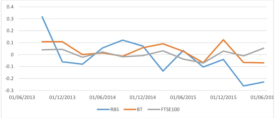
Figure 6 – The volatilities of the underlying (option portfolio)

1,000 2,000 3,000 4,000 5,000

1 Day VaR (99%) 5 Days VaR (99%) 1 Day VaR (95%) 5 Days VaR (95%)

Option Portfolio VaR

Delta-normal Delta-gamma Historical Monte Carlo

-0.3 -0.2 -0.1 0 0.1 0.2 0.3 0.4

01/06/2013 01/12/2013 01/06/2014 01/12/2014 01/06/2015 01/12/2015 01/06/2016

[image:34.595.70.525.542.738.2]

(35)

35 The gamma

[image:35.595.76.526.371.563.2]

An important variable to be analysed is the gamma, the rate of change in delta when the price of the underlying asset changes. Figure 7 illustrates the gamma behaviour of the call option with the underlying RBS and strike price £160 versus the hypothetical stock price as time to maturity decreases. The long call position is in the money (ITM), that is when the price of the underlying stock of a long call is higher than the strike price. Options that are in the money and close to the expiration have very high gammas. So, the option price is highly sensitive to changes in price of the underlying asset. On the other hand, when options are out the money (OTM) or have a further expiration date, they have lower gammas. In the option portfolio analysed here, there are two ITM options (underlying BT and RBS stocks) and one OTM option (underlying FTSE 100 index). This comparison is demonstrated in Table 4. Following the theory, the higher gammas in the portfolio are from the ITM options. As the weight invested in each option is equal, the impact of the gamma in the portfolio tends to increase the delta gamma VaR. Clearly, the higher gammas are from underlying assets with higher standard deviation according to the equation (5).

Figure 7 – Call option gamma x underlying stock price

Position Underlying Gamma Standard Deviation

ITM Long call RBS stock 0.86% 33.90%

ITM Long put BT stock 0.51% 22.62%

OTM Long call FTSE 100 index 0.06% 15.30%

Table 4 – The gamma of the underlying (option portfolio)

0.02 0.04 0.06 0.08 0.10 0.12 0.14 0.16

70 90 110 130 150 170 190 210 230 250

Gamma x Stock price

[image:35.595.71.532.600.659.2]

(36)

36 The correlation

According to the theory, there is a gain in the risk measure when considering a portfolio compound by correlated instruments. The correlation between financial instruments represents how they react between themselves to the market price movements, positively or negatively and the magnitude of this movement. Meucci (2010) demonstrates the benefits and performance of diversification in market risk measures.

Figure 8 shows the comparison between the diversified and non-diversified option portfolio VaR for the delta normal and gamma, historical and Monte Carlo models. The blue bars represent the VaR of a non-diversified portfolio and the orange bars the non-diversified portfolios. The Monte Carlo simulation presents higher efficiency with diversification as it has larger difference between undiversified and diversified VaR portfolios. On the other hand, the delta gamma is less efficient in considering correlation in the risk measure.

[image:36.595.69.502.448.658.2]

It is clear the benefits of the diversification due to the interaction of the underlying stock prices with different risk factors. In the undiversified portfolio the options are totally correlated then, the portfolio VaR is simply the sum of the individual option VaRs. The higher the correlation, the lower the difference between the undiversified and diversified portfolios. The correlation between the options of this portfolio is an advantage as it can limit or stop the loss of money with unexpected change in prices.

Figure 8 - The 1 day (99%) VaR for the undiversified and diversified option portfolio.

500 1,000 1,500 2,000 2,500

Delta-normal Delta-gamma Historical Monte Carlo

Undiversified/diversified portfolio VaR

(37)

37 4.3 Results comparison

In the historical simulation, the VaR is totally based upon time series of past returns. Consequently, it can underestimate the VaR whether the historical data is stable or overestimate the VaR when the historical data is not stable. The results showed that both portfolios analysed in this study are highly liquid and volatile. For these 2 portfolios, the historical simulation is not a good indicator of forecasting losses. Boudoukh et al. (1998), Hull and White (1998) propose alternative models based on historical simulation that leads with the problem of outliers in the return distribution by weighting the data.

Regarding the delta normal VaR, this is heavily based on the standard deviation of the returns and consequently, it has a normal distribution. However, catastrophic events are quite likely to happen according to the financial historical facts. Engle (2001) suggests a more accurate VaR calculation when considering possible changes in the standard deviation over time. Also, volatile instruments can have outliers in their return distribution that might make the normal distribution inapplicable. It is clear that the delta normal VaR cannot be considered the best outfit model for the stock portfolio. For the option portfolio analysed, the higher delta normal VaR is more conservative in terms of estimating the expected loss because it does not consider the non-linear premise of options. So, this is not applicable to the option portfolio.

For both portfolios, the Monte Carlo simulations show to be a more flexible and fair method to estimate the VaR. The consistent results for portfolios with different peculiarities illustrate the flexibility and preference of this model among financial institutions. On the other hand, Jamshidian and Zhu (1997), Frye (1997), Glasserman et al. (2000) and Botev et al. (2010) suggest improvements in Monte Carlo to deal with the computational time required to simulate plenty of random scenarios to compute the VaR.

The delta-gamma model also seems to be an accurate measure for the option portfolio allowing to estimate the VaR for the non-linear instruments. However, this method requires mathematics so intensively that can become extremely complicated and costly to some institutions. Despite most literature recommending the delta-gamma approach for leading with non-linearity, Castellacci and Siclari (2003) find a more precise measure in the delta normal than in the delta gamma method for non-linear option portfolios.

4.4 Advantages and weaknesses of the VaR methods