Updating QR factorization procedure for solution of linear least squares problem with equality constraints

R E S E A R C H

Open Access

Updating

QR

factorization procedure for

solution of linear least squares problem with

equality constraints

Salman Zeb

_{and Muhammad Yousaf}

*_{Correspondence:}

[email protected] Department of Mathematics, University of Malakand, Dir (Lower), Chakdara, Khyber Pakhtunkhwa, Pakistan

Abstract

In this article, we present aQRupdating procedure as a solution approach for linear least squares problem with equality constraints. We reduce the constrained problem to unconstrained linear least squares and partition it into a small subproblem. TheQR factorization of the subproblem is calculated and then we apply updating techniques to its upper triangular factorRto obtain its solution. We carry out the error analysis of the proposed algorithm to show that it is backward stable. We also illustrate the implementation and accuracy of the proposed algorithm by providing some numerical experiments with particular emphasis on dense problems.

MSC: 65-XX; 65Fxx; 65F20; 65F25

Keywords: QRfactorization; orthogonal transformation; updating; least squares problems; equality constraints

1 Introduction

We consider the linear least squares problem with equality constraints (LSE)

min

x Ax–b, subject toBx=d, ()

whereA∈Rm×n_,b∈Rm_,B∈Rp×n_,d∈Rp_,x∈Rn_{withm+p≥n≥pand ·}

denotes the

Euclidean norm. It arises in important applications of science and engineering such as in beam-forming in signal processing, curve fitting, solutions of inequality constrained least squares problems, penalty function methods in nonlinear optimization, electromagnetic data processing and in the analysis of large scale structure [–]. The assumptions

rank(B) =p and null(A)∩null(B) ={} ()

ensure the existence and uniqueness of solution for problem ().

The solution of LSE problem () can be obtained using direct elimination, the nullspace method and method of weighting. In direct elimination and nullspace methods, the LSE problem is first transformed into unconstrained linear least squares (LLS) problem and then it is solved via normal equations orQRfactorization methods. In the method of weighting, a large suitable weighted factorγ is selected such that the weighted residual

γ(d–Bx) remains of the same size as that of the residual b–Ax and the constraints is satisfied effectively. Then the solution of the LSE problem is approximated by solv-ing the weighted LLS problem. In [], the author studied the method of weightsolv-ing for LSE problem and provided a natural criterion of selecting the weighted factorγ such that

γ ≥ A/BM, whereMis the rounding unit. For further details as regards methods

of solution for LSE problem (), we refer to [, , , –].

Updating is a process which allow us to approximate the solution of the original problem without solving it afresh. It is useful in applications such as in solving a sequence of mod-ified related problems by adding or removing data from the original problem. Stable and efficient methods of updating are required in various fields of science and engineering such as in optimization and signal processing [], statistics [], network and structural anal-ysis [, ] and discretization of differential equations []. Various updating techniques based on matrix factorization for different kinds of problems exist in the literature [, , , –]. Hammarling and Lucas [] discussed updating theQRfactorization with ap-plications to LLS problem and presented updating algorithms which exploited LEVEL  BLAS. Yousaf [] studied repeated updating based onQRfactorization as a solution tool for LLS problem. Parallel implementation on GPUs of the updatingQRfactorization algo-rithms presented in [] is performed by Andrew and Dingle []. Zhdanov and Gogoleva [] studied augmented regularized normal equations for solving LSE problems. Zeb and Yousaf [] presented an updating algorithm by repeatedly updating both factors of the

QRfactorization for the solutions of LSE problems.

In this article, we consider the LSE problem () in the following form:

min

x(γ)

γB A

x–

γd

b



, ()

which is an unconstrained weighted LLS problem whereγ ≥ A/BM given in []

and approximated its solution by updating HouseholderQRfactorization. It is well known that HouseholderQRfactorization is backward stable [, , , ]. The conditions given in () ensure that problem () is a full rank LLS problem. Hence, there exist a unique so-lutionx(γ) of problem () which approximated the solutionxLSEof the LSE problem ()

such thatlimγ→∞x(γ) =xLSE. In our proposed technique, we reduced problem () to a

small subproblem using a suitable partitioning strategy by removing blocks of rows and columns. TheQRfactorization of the subproblem is calculated and its Rfactor is then updated by appending the removed block of columns and rows, respectively, to approxi-mate the solution of problem (). The presented approach is suitable for solution of dense problems and also applicable for those applications where we are adding new data to the original problem andQRfactorization of the problem matrix is already available.

We organized this article as follows. Section  contains preliminaries related to our main results. In Section , we present theQRupdating procedure and algorithm for solution of LSE problem (). The error analysis of the proposed algorithm is provided in Section . Numerical experiments and comparison of solutions is given in Section , while our con-clusion is given in Section .

2 Preliminaries

2.1 The method of weighting

This method is based on the observations that while solving LSE problem () we are inter-ested that some equations are to be exactly satisfied. This can be achieved by multiplying large weighted factorγ to those equations. Then we can solve the resulting weighted LLS problem (). The method of weighting is useful as it allows for the use of subroutines for LLS problems to approximate the solution of LSE problem. However, the use of the large weighted factorγ can compromise the conditioning of the constrained matrix. In partic-ular, the method of normal equations when applied to problem () fails for large values of

γ in general. For details, see [, –].

2.2 QRfactorization and householder reflection

Let

X=QR ()

be theQRfactorization of a matrixX∈Rm×nwhereQ∈Rm×mandR∈Rm×n. This fac-torization can be obtained using Householder reflections, Givens rotations and the

classi-cal/modified Gram-Schmidt orthogonalization. The Householder and GivensQR

factor-ization methods are backward stable. For details as regardsQRfactorization, we refer to [, ].

Here, we briefly discuss the Householder reflection method due to our requirements. For a non-zero Householder vectorv∈Rn_{, we define the matrixH∈R}n×n_as

H=In–τvvT, τ =



vT_v, ()

which is called the Householder reflection or Householder matrix. Householder matrices are symmetric and orthogonal. For a non-zero vectoru, the Householder vectorvis simply defined as

v=u± uek,

such that

Hu=u–τvvTu=∓αek, ()

whereα=uandekdenotes thekth unit vector inRnin the following form:

ek(i) = ⎧ ⎨ ⎩

 ifi=k,

 otherwise.

In our present work given in next section, we will use the following algorithm for compu-tation of Householder vectorv. This computation is based on Parlett’s formula []:

v=u–u=

u–u

x+u

= –u

 

u+u

,

whereu>  is the first element of the vectoru∈Rn. Then we compute the Householder

Algorithm Computation of parameterτ and Householder vectorv[] Input: u,u

Output: v,τ

: α=u_

: v=u,v() = 

: if(α= ) then

: τ= 

: else

: β=u_+α

: end if

: ifu≤ then : v() =u–β : else

: v() = –α/(u+β) : end if

: τ = v()_/(α+v()₎ : v=v/v()

3 UpdatingQRfactorization procedure for solution of LSE problem

Let

E=

γB

A

∈R(m+p)×n and f=

γd

b

∈Rm+p.

Then we can write problem () as

min

x(γ)Ex–f. ()

Here, we will reduce problem () to a small incomplete subproblem using suitable parti-tion process. In partiparti-tion process, we remove blocks of rows and columns from the prob-lem matrixEconsidered in () and from its corresponding right-hand side (RHS) without involving any arithmetics. That is, we consider

E=

⎛ ⎜ ⎝

E( :j– ,  :n)

E(j:j+r,  :n)

E(j+r+  :m+p,  :n)

⎞ ⎟

⎠ and f =

⎛ ⎜ ⎝

f( :j– )

f(j:j+r)

f(j+r+  :m+p)

⎞ ⎟

⎠, ()

and removing blocks of rows from bothEandf in equation () as

Gr=E(j:j+r,  :n)∈Rr×n and fr=f(j:j+r), ()

we get

E=

E( :j– ,  :n)

E(j+r+  :m+p,  :n)

, f=

f( :j– )

f(j+r+  :m+p)

Algorithm Calculating theQRfactorization and computing matrixUc

Input: E∈Rm×n,f∈Rm,Gc∈Rm×c

Output: R∈Rm×n,g∈Rm,Uc∈Rm×c

: R←−E

: fork=  to min(m,n) do

: [v,τ,E(k,k)] =house(E(k,k),E(k+  :m,k)) : V=E(k,k+  :n) +vTE(k+  :m,k+  :n) : R(k,k+  :n) =E(k,k+  :n) –τV

: ifk<nthen

: R(k+  :m,k+  :n) =E(k+  :m,k+  :n) –τvV : end if

: g(j:m) =f(k:m) –τ



v

vT_f(k:m)

: Uc(k:m,k:end) =Gc(k:m,k:end) –τ

_ v

vT_U

c(k:m,k:end) : end for

Hence, we obtain the following problem:

min

x

Ex–f, E∈Rm×n,f∈Rm,x∈Rn, ()

wherem=m+p–r,n=n, andfr∈Rr. Furthermore, by removing block of columns

Gc=E(:,j:j+c) from thejth position by considering the partition ofEin the incomplete

problem () as

E=

E(:,  :j– ) E(:,j:j+c) E(:,j+c+  :n)

, ()

we obtain the following reduced subproblem:

min

x

Ex–f, E∈Rm×n,f∈Rm,x∈Rn, ()

whereE= [E(:,  :j– ),E(:,j+  :n)],n=n–c,m=m, andf=f.

Now, we calculated theQRfactorization of the incomplete subproblem () is order to reduce it to the upper triangular matrixRusing the following algorithm (Algorithm ).

Herehousedenotes the Householder algorithm and the Householder vectors are calcu-lated using Algorithm  andVis a self-explanatory intermediary variable.

Hence, we obtain

R=Hn· · ·HE, g=Hn· · ·Hf ()

and

Uc=Hn· · ·HGc.

Here, theQRfactorization can also be obtained directly using the MATLAB built-in com-mandqrbut it is not preferable due to its excessive storage requirements for orthogonal matrixQand by not necessarily providing positive sign of diagonal elements in the matrix

Algorithm UpdatingRfactor after appending a block of columnsGc

Input: R∈Rm×n,Gc∈Rm×c,g∈Rm

Output: R∈Rm×(n+c),g∈Rm

: Gc( :m,  :c)←−R( :m,n+  :n+c) : if(m≥n) then

: R←−triu(R) : g←−g : else

: fork=jto min(m,n+c) do

: [v,τ,R(k,k)] =house(R(k,k),R(k+  :m,k)) : V=R(k,k+  :n+c) +vTR(k+  :m,k+  :n+c)) : R(k,k+  :n+c) =R(k,k+  :n+c) –τV

: ifk<n+cthen

: R(k+  :m,k+  :n+c) =R(k+  :m,k+  :n+c) –τvV : end if

: g(k:m) =g(k:m) –τ



v

vTg(k:m) : end for

: R= triu(R) : end if

To obtain the solution of problem (), we need to update the upper triangular matrix

R. For this purpose, we append the updated block of columnsGcto theRfactor in ()

at thejth position as follows:

Rc=

R(:,  :j– ) Gc(:,j:j+c) R(:,j+c+  :n)

. ()

Here, if theRcfactor in () is upper trapezoidal or in upper triangular form then no

further calculation is required, and we getR=Rc. Otherwise, we will need to reduce

equation () to the upper triangular factorRby introducing the Householder matrices

Hn+c, . . . ,Hj:

R=Hn+c· · ·HjRc and g=Hn+c· · ·Hjg, ()

whereR∈Rm×nis upper trapezoidal form<nor it is an upper triangular matrix. The

procedure for appending the block of columns and updating of theRfactor in algorithmic

form is given as follows (Algorithm ).

Here the term triu denotes the upper triangular part of the concerned matrix andVis the intermediary variable.

Now, we append a block of rowsGrto theRfactor andfrto its corresponding RHS at

thejth position in the following manner.

Rr= ⎛ ⎜ ⎝

R( :j– , :)

Gr( :r, :)

R(j:m, :)

⎞ ⎟

⎠, gr= ⎛ ⎜ ⎝

g( :j– )

fr( :r)

g(j:m)

Algorithm UpdatingRfactor after appending a block of rowsGr

Input: R∈Rm×n,Gr∈Rr×n,g∈Rm,fr∈Rm

Output: R˜∈R(m+r)×n_,g˜∈Rm+r

: fork=  to min(m,n) do

: [v,τ,R(k,k)] =house(R(k,k),Gr( :r,k))

: V=R(k,k+  :n) +vTGr( :r,k+  :n)

: R˜(k,k+  :n) =R(k,k+  :n) –τV : ifk<nthen

: Gr( :r,k+  :n) =Gr( :r,k+  :n) –τvV

: end if

: gk=g(k)

: g(k)≡( –τ)g(k) –τvT_f r( :r)

: fr( :r)≡fr( :r) –τvgk–τvvTfr( :r)

: end for

: ifm<nthen

: [Qr,Rr] =qr(Gr(:, (m+  :n))) : Rr(m+  :m+r,m+  :n)←− ˜Rr

: fr≡QTrfr

: end if

: R˜←−_R

: g˜←−_fg_r

We use the permutation matrixP in order to bring the block of rowsGr andfr at the

bottom position if required. Then

PRr=

R

Gr

, Pgr=

g

fr

. ()

The equation () is reduced to upper triangular form by constructing the matrices

H, . . . ,Hnusing Algorithm  as given by

˜

R=HnHn–· · ·H

R

Gr

and

˜

g=HnHn–· · ·H

g

fr

.

The procedure is performed in algorithmic form as follows (Algorithm ).

Hereqris the MATLAB command ofQRfactorization andV is a self-explanatory

in-termediary variable.

The solution of problem () can then be obtained by applying the MATLAB built-in

commandbacksubfor a back-substitution procedure.

Algorithm UpdatingQRalgorithm for solution of LSE problem Input: A∈Rm×n_,b∈Rm_,B∈Rp×n_,d∈Rp

Output: xLSE∈Rn : E=γ_ABandf =γd

b

: [E,f,Gr,E,Gc,fr]←−partition(E,f)

: [R,g,Uc]←−QRfactorization of subproblem (E,f,Gc)

: [R,g]←−appendbcols(R,g,Uc)

: [R˜,g˜]←−appendbrows(R,Gr,g,fr)

: xLSE←−backsub(R˜( :n,  :n),g˜( :n))

Here, Algorithm  for a solution of LSE problem () calls upon the partition process,

Algorithms , ,  and MATLAB commandbacksubfor back-substitution procedure,

re-spectively.

4 Error analysis

In this section, we will study the backward stability of our proposed Algorithm . The mainstay in our presented algorithm for the solution of LSE problem is the updating pro-cedure. Therefore, our main concern is to study the error analysis of the updating steps. For others, such as the effect of using the weighting factor, finding theQRfactorization and for the back-substitution procedure, we refer the reader to [, ]. Here, we recall some important results without giving their proofs and refer the reader to [].

We will consider the following standard model of floating point arithmetic in order to analyze the rounding errors effects in the computations:

fl(xopy) = (xopy)( +η), |η| ≤M, op = +, –,∗, /, ()

whereMis the unit roundoff. The value ofMis of order –in single precision computer

arithmetic, while in double precision it is of the order –_{. Moreover, for addition and}

subtraction in the absence of guard integers, we can write model () as follows:

fl(x±y) =x( +η)±y( +η), |ηi| ≤M, i= , .

Lemma .([]) If|ηi| ≤M,δi=±for i= , , . . . ,n and nM< ,then n

i=

( +ηi)δi=  +φn,

where

|φn| ≤

nM

 –nM

=γn.

Here, we will use the constantsγnandγ˜cnfor convenience as adopted in [] where these

are defined by

γn=

nM

 –nM

and

˜ γcn=

ncM

 –ncM

, assumingncM< , ()

wherecis a small positive integer.

Lemma .([]) Let x,y∈Rn_{and consider the inner product x}T_y.Then

flxTy=xT(y+y), |y| ≤γn|y|.

Lemma .([]) Letφk andγkbe defined for any positive integer k.Then for positive

integers j and k the following relations hold:

( +φk)( +φj) =  +φk+j, ()

( +φk)

( +φj)

=

⎧ ⎨ ⎩

 +φk+j, j≤k,

 +φk+j, j>k,

()

jγk≤γjk, ()

kγk+M≤γk+, ()

γk+γj+γkγj≤γk+j. ()

Lemma .([]) Considering the construction ofτ ∈Rand v∈Rn_{given in Section,}

then the computedτ˜andv in floating point arithmetic satisfy˜

˜

v( :n) =v( :n)

and

˜

τ=τ( +φ˜n) and v˜=v( +φ˜n),

whereφ˜n≤ ˜γn.

Here, we represent the Householder transformation asI–vvT, which requiresv=

√ . Therefore, by redefiningv=√τvandτ=  using Lemma ., we have

˜

v=v+v, |v| ≤ ˜γmv forv∈Rm,v=

√

. ()

Lemma .([]) Considering the computation of y=Hb˜ = (I–˜vv˜T_{)b=b–v˜(v˜}T_b)for

b∈Rm_andv˜∈Rm_{satisfies().Then the computedy satisfies˜} ˜

y= (H+H)b, HF≤ ˜γm,

where H=I–vvT_{and ·}

Lemma .([]) Let Hk=I–vkvTk ∈Rm×mbe the Householder matrix and we define the

sequence of transformations

Xk+=HkXk, k=  :r,

where X=X∈Rm×n.Furthermore,it is assumed that these transformations are performed

using computed Householder vectorsv˜k≈vkand satisfy Lemma..Then we have ˜

Xr+=QT(X+X), ()

where QT_=H

r, . . . ,H,and

xj≤rγ˜mxj, j=  :n.

Theorem .([]) LetR˜∈Rm×n_{be the computed upper trapezoidal QR factor of X∈} Rm×n_{(m≥n)obtained via Householder QR algorithm by Lemma..Then there exists}

an orthogonal matrix Q∈Rm×m_{such that}

X+X=QR˜,

where

xj≤ ˜γmnxj, j=  :n. ()

Lemma .([]) Let X∈Rm×n_{and H=I–τvv}T_∈Rm×m _{be the Householder matrix.}

Also,assuming that the computation of HX is performed using computedτ˜andv such that˜ it satisfies Lemma..Then,from Theorem.,we have

fl(HX) =H(X+X), XF≤γcmXF. ()

4.1 Backward error analysis of proposed algorithm

To appreciate the backward stability of our proposed Algorithm , we first need to carry out the error analysis of Algorithms  and . For this purpose, we present the following.

Theorem . The computed factorR in Algorithm˜ satisfies

˜

R=QT

R

Gr

+er

and erF≤ ˜γn(r+)

R

Gr

F

,

where Gr∈Rr×nis the appended block of rows to the Rfactor and Q=HH· · ·Hn.

Proof Let the Householder matrixHjhave zeros on thejth column of the matrix ˜rjj

Grj

. Then using Lemma ., we have

H

R

Gr

+e

=

˜

Rr ˜

Gr

where

eF≤ ˜γr+

R Gr F . Similarly, H ˜

Rr ˜

Gr

+e

=

˜

Rr ˜

Gr

=HH

R

Gr

+e()_r

,

and

eF≤ ˜γr+

˜

Rr ˜

Gr F , where _e()

r F=e+eF, e()_{r F}≤ eF+eF,

≤ ˜γr+

R Gr F

+γ˜r+

ˆ

Rr ˆ

Gr

F

.

From equation (), we have

ˆ

Rr ˆ

Gr F ≤ R Gr F

+e

≤ R Gr F

+γ˜r+

R Gr F .

This implies that

_e()

r F≤ ˜γr+ R Gr F

+γ˜r+( +γ˜r+)

R Gr F

≤γ˜r++γ˜r+( +γ˜r+)

R Gr F

≤γ˜r+

R Gr F ,

where we ignored (γ˜r+)asγ˜r+is very small.

Continuing in the same fashion till thenth Householder reflection, we have

˜

R=HnHn–· · ·H

R

Gr

+er

where

erF=er(n)F≤nγ˜r+

R

Gr

F

,

or, by using equation () of Lemma ., we can write

erF≤ ˜γn(r+)

R

Gr

F

,

which is the required result.

Theorem . The backward error for the computed factor Rin Algorithmis given by

R=Q˜T

(R,Uc) +e˜c

,

where Uc∈R(m+p)×cis the appended block of columns to the right-end of Rfactor,˜ecF≤ ˜

γ(m+p)cUcFandQ˜ =Hn+· · ·Hn+c.

Proof To prove the required result, we proceed similar to the proof of Theorem ., and obtain

e_cF≤γ˜c(R,Uc) +e˜c_F.

This implies that the error in the whole process of appending the block of columns to the

Rfactor is given by

R=Hn+c· · ·Hn+

(R,Uc) +e˜c

,

where

ecF≤ ˜γ(m+p)cUcF.

Theorem . Let the LSE problem()satisfy the conditions given in().Then Algorithm

solves the LSE problem with computedQ˜ =H· · ·HnandR which satisfies˜ I–Q˜T_Q˜

F≤ √

nγ˜(m+p)n ()

and

E–Q˜R˜F≤ √

nγ˜(m+p)nEF. ()

Proof To study the backward error analysis of Algorithm , we consider the reduced sub-problem matrixE∈Rm×n from () and letˆebe its backward error in the computed

QRfactorization. Then from Lemma ., we have

As in our proposed Algorithm , we appended a block of columnsUc=QTGcto theR

factor, then by using Theorem ., we have

R=Hn+· · ·Hn+c

(R,Uc) +ec

,

whereecF≤ ˜γmcUcF.

Therefore, by simplifying

ˆeF=QTQTˆe+QTec_F,

whereQT =Hn+· · ·Hn+candˆeis the error of computing theQRfactorization, we obtain

ˆeF=QTQTˆe+QTec_F

≤QT_FQT_FˆeF+QTFecF ≤ ˆeF+ecF

≤ ˜γmnEF+γ˜mcUcF

≤[γ˜mn+γ˜mc]max

EF,UcF

.

Hence, we have

ˆeF≤[γ˜mn+γ˜mc]max

EF,UcF

,

which is the total error at this stage of appending the block of columns and its updating. Furthermore, we appended the block of rowsGr to the computed factorR in our

algo-rithm and, by using Theorem ., we obtain

˜

R=Hn· · ·H

R

Gr

+er

,

where

erF≤ ˜γ(r+)n

R

Gr

F

,

is the error for appending the block of rowsGr.

Hence, the total errorefor the whole updating procedure in Algorithm  can be written as

eF≤ erF+ˆeF ≤ ˜γ(r+)n

R

Gr

F

+ (γ˜mn+γ˜mc)max

EF,UcF

≤(γ˜(r+)n+γ˜mn+γ˜mc)max

EF,UcF,

R

Gr

F

Now, if the orthogonal factorQis to be formed explicitly, then the deviation from nor-mality in our updating procedure can be examined. For this, we considerE=I, then from Lemma ., we have

˜

Q=QT(Im+ζ),

whereζ is the error in the computed factorQ˜given as

ζF≤ ˜γmnImF=

√

nγ˜mn,

where ImF =

√

n. In a similar manner, the computed factor Q˜ after appending

columnsUcis given by ˜

Q=QT(Im+ζc),

where

ζcF≤ √

cγ˜mc.

Therefore, the total error inQ˜ is given as ˜

QQ˜=QT(Im+ζ),

where

ζF≤ ζF+ζcF≤ √

nγ˜mn+

√

cγ˜mc.

Similarly, the error in the computed factorQ˜ after appending block of rows is given as ˜

Q=QT(Ir+ζr),

where

ζrF≤ √

nγ˜(r+)n.

So, the total errorζinQduring the whole updating procedure is given by ζF=ζF+ζrF

≤√nγ˜(r+)n+√nγ˜mn+

√

cγ˜mc, ()

wherem<m+p,n<nandc<n.

Therefore, the error measure inQ˜ which shows the amount by which it has been devi-ated from normality is given by

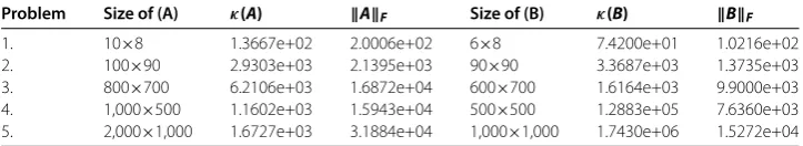
Table 1 Description of test problems

Problem Size of (A) κ(A) AF Size of (B) κ(B) BF

1. 10×8 1.3667e+02 2.0006e+02 6×8 7.4200e+01 1.0216e+02 2. 100×90 2.9303e+03 2.1395e+03 90×90 3.3687e+03 1.3735e+03 3. 800×700 6.2106e+03 1.6872e+04 600×700 1.6164e+03 9.9000e+03 4. 1,000×500 1.1602e+03 1.5943e+04 500×500 1.2883e+05 7.6360e+03 5. 2,000_×1,000 1.6727e+03 3.1884e+04 1,000_×1,000 1.7430e+06 1.5272e+04

From equation (), we have

˜

γ(r+)n+γ˜mn+γ˜mc≈ ˜γ(m+p+)n=γ˜(m+p)n, ()

and using it in equation (), we get the required result (). Also, we have

E–Q˜R˜F=(E–QR˜) +

(Q–Q˜)R˜_F

≤√n(γ˜(r+)n+γ˜mn+γ˜mc)max

EF,EcF,

R

Gr

F

. ()

AsXF=QRF=RF, therefore, we can write

max

EF,UcF,

R

Gr

F

=

R

Gr

F

=EF. ()

Hence, applying expressions () and () to (), we obtain the required equation ()

which shows how large is the error in the computedQRfactorization.

5 Numerical experiments

This section is devoted to some numerical experiments which illustrate the

applicabil-ity and accuracy of Algorithm . The problem matricesAandBand its corresponding

right-hand side vectorsbanddare generated randomly using the MATLAB built-in

com-mandsrand(‘twister’) andrand. These commands generate pseudorandom numbers from

a standard uniform distribution in the open interval (, ). The full description of test matrices are given in Table , where we denote the Frobenius norm with · F and the

condition number byκ(·). For accuracy of the solution, we consider the actual solution such thatx=rand(n, ) and denote the result obtained from Algorithm  byxLSEand that

of directQRHouseholder factorization with column pivoting byxp. We obtain the

rela-tive errors between the solutions given in Table . Moreover, the solutionxLSEsatisfy the

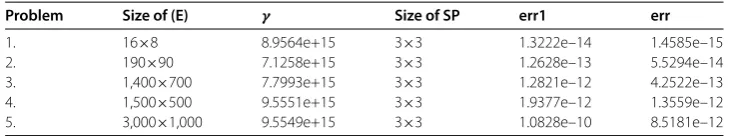
constrained system effectively. The description of the matrixE, the size of the reduced subproblem (SP), value of the weighted factorω, the relative errorserr=x–xLSE/x

anderr1=x–xp/xare provided in Table . We also carry out the backward error

tests of Algorithm  numerically for our considered problems and provide the results in Table , which agrees with our theoretical results.

6 Conclusion

The solution of linear least squares problems with equality constraints is studied by

Table 2 Results comparison

Problem Size of (E) γ Size of SP err1 err

1. 16×8 8.9564e+15 3×3 1.3222e–14 1.4585e–15 2. 190×90 7.1258e+15 3×3 1.2628e–13 5.5294e–14 3. 1,400×700 7.7993e+15 3×3 1.2821e–12 4.2522e–13 4. 1,500×500 9.5551e+15 3×3 1.9377e–12 1.3559e–12 5. 3,000×1,000 9.5549e+15 3×3 1.0828e–10 8.5181e–12

Table 3 Backward error analysis results

Problem E–Q˜R˜F

EF I –Q˜ T_Q˜

F

1. 4.4202e–16 1.3174e–15 2. 4.7858e–16 9.0854e–15 3. 1.0450e–15 4.9428e–14 4. 9.0230e–16 3.8711e–14 5. 9.9304e–16 6.4026e–14

factorization of the small subproblem in order to obtain the solution of our considered problem. Numerical experiments are provided which illustrated the accuracy of the pre-sented algorithm. We also showed that the algorithm is backward stable. The prepre-sented approach is suitable for dense problems and also applicable whereQRfactorization of a problem matrix is available and we are interested in the solution after adding new data to the original problem. In the future, it will be of interest to study the updating techniques for sparse data problems and for those where the linear least squares problem is fixed and the constraint system is changing frequently.

Competing interests

The authors declare that they have no competing interests.

Authors’ contributions

All authors contributed equally to this work. All authors read and approved the final manuscript.

Publisher’s Note

Springer Nature remains neutral with regard to jurisdictional claims in published maps and institutional affiliations.

Received: 5 July 2017 Accepted: 16 October 2017

References

1. Auton, JR, Van Blaricum, ML: Investigation of procedures for automatic resonance extraction from noisy transient electromagnetics data. Final Report, Contract N00014-80-C-029, Office of Naval Research Arlington, VA 22217 (1981) 2. Barlow, JL, Handy, SL: The direct solution of weighted and equality constrained least-squares problems. SIAM J. Sci.

Stat. Comput.9, 704-716 (1988)

3. Lawson, CL, Hanson, RJ: Solving Least Squares Problems. SIAM, Philadelphia (1995)

4. Eldén, L: Perturbation theory for the least squares problem with linear equality constraints. SIAM J. Numer. Anal.17, 338-350 (1980)

5. Leringe, O, Wedin, PÅ: A comparison between different methods to compute a vectorxwhich minimizesAx–b2

whenGx=h. Tech. Report, Department of computer science, Lund University (1970)

6. Van Loan, CF: A generalized SVD analysis of some weighting methods for equality constrained least squares. In: Kågström, B, Ruhe, A (eds.) Matrix Pencils. Lecture Notes in Mathematics, vol. 973, pp. 245-262. Springer, Heidelberg (1983)

7. Van Loan, CF: On the method of weighting for equality-constrained least-squares problems. SIAM J. Numer. Anal.22, 851-864 (1985)

8. Wei, M: Algebraic properties of the rank-deficient equality-constrained and weighted least squares problems. Linear Algebra Appl.161, 27-43 (1992)

9. Stewart, GW: On the weighting method for least squares problems with linear equality constraints. BIT Numer. Math. 37, 961-967 (1997)

10. Anderson, E, Bai, Z, Dongarra, J: GeneralizedQRfactorization and its applications. Linear Algebra Appl.162, 243-271 (1992)

12. Golub, GH, Van Loan, CF: Matrix Computations. Johns Hopkins University Press, Baltimore (1996) 13. Stewart, GW: Matrix Algorithms. SIAM, Philadelphia (1998)

14. Alexander, ST, Pan, CT, Plemmons, RJ: Analysis of a recursive least squares hyperbolic rotation algorithm for signal processing. Linear Algebra Appl.98, 3-40 (1988)

15. Chambers, JM: Regression updating. J. Am. Stat. Assoc.66, 744-748 (1971)

16. Haley, SB, Current, KW: Response change in linearized circuits and systems: computational algorithms and applications. Proc. IEEE73, 5-24 (1985)

17. Haley, SB: Solution of modified matrix equations. SIAM J. Numer. Anal.24, 946-951 (1987)

18. Lai, SH, Vemuri, BC: Sherman-Morrison-Woodbury-formula-based algorithms for the surface smoothing problem. Linear Algebra Appl.265, 203-229 (1997)

19. Björck, Å, Eldén, L, Park, H: Accurate downdating of least squares solutions. SIAM J. Matrix Anal. Appl.15, 549-568 (1994)

20. Daniel, JW, Gragg, WB, Kaufman, L, Stewart, GW: Reorthogonalization and stable algorithms for updating the Gram-SchmidtQRfactorization. Math. Comput.30, 772-795 (1976)

21. Gill, PE, Golub, GH, Murray, W, Saunders, M: Methods for modifying matrix factorizations. Math. Comput.28, 505-535 (1974)

22. Reichel, L, Gragg, WB: Algorithm 686: FORTRAN subroutines for updating theQRdecomposition. ACM Trans. Math. Softw.16, 369-377 (1990)

23. Hammarling, S, Lucas, C: Updating theQRfactorization and the least squares problem. Tech. Report, The University of Manchester (2008). http://www.manchester.ac.uk/mims/eprints

24. Yousaf, M: Repeated updating as a solution tool for linear least squares problems. Dissertation, University of Essex (2010)

25. Andrew, R, Dingle, N: ImplementingQRfactorization updating algorithms on GPUs. Parallel Comput.40, 161-172 (2014)

26. Zhdanov, AI, Gogoleva, SY: Solving least squares problems with equality constraints based on augmented regularized normal equations. Appl. Math. E-Notes15, 218-224 (2015)

27. Zeb, S, Yousaf, M: RepeatedQRupdating algorithm for solution of equality constrained linear least squares problems. Punjab Univ. J. Math.49, 51-61 (2017)

28. Higham, NJ: Accuracy and Stability of Numerical Algorithms. SIAM, Philadelphia (2002)

29. Wilkinson, JH: Error analysis of transformations based on the use of matrices of the formI– 2wwH_{. In: Rall, LB (ed.)}

Error in Digital Computation, vol. 2, pp. 77-101. Wiley, New York (1965)

30. Parlett, BN: Analysis of algorithms for reflections in bisectors. SIAM Rev.13, 197-208 (1971)