Comparison and analysis of two forms of harvesting functions in the two prey and one predator model

R E S E A R C H

Open Access

Comparison and analysis of two forms

of harvesting functions in the two-prey

and one-predator model

Xinxin Liu

_{and Qingdao Huang}

*_{Correspondence:} [email protected] 1_{School of Mathematics (Zhuhai),}

Sun Yat-sen University, Zhuhai, China

2_{School of Mathematics, Jilin}

University, Changchun, China

Abstract

A new way to study the harvested predator–prey system is presented by analyzing the dynamics of two-prey and one-predator model, in which two teams of prey are interacting with one team of predators and the harvesting functions for two prey species takes different forms. Firstly, we make a brief analysis of the dynamics of the two subsystems which include one predator and one prey, respectively. The positivity and boundedness of the solutions are verified. The existence and stability of seven equilibrium points of the three-species model are further studied. Specifically, the global stability analysis of the coexistence equilibrium point is investigated. The problem of maximum sustainable yield and dynamic optimal yield in finite time is studied. Numerical simulations are performed using MATLAB from four aspects: the role of the carrying capacity of prey, the simulation about the model equations around three biologically significant steady states, simulation for the yield problem of model system, and the comparison between the two forms of harvesting functions. We obtain that the new form of harvesting function is more realistic than the traditional form in the given model, which may be a better reflection of the role of human-made disturbance in the development of the biological system.

MSC: 34D20; 49M30; 92B05

Keywords: Three species model; Harvesting function; Maximum sustainable yield; Global stability

1 Introduction

The interaction between the predator and prey is one of basic relationships among bio-logical species, which becomes one of the hot issues in ecology and biomathematics. The predator–prey model is widely used in renewable resources management [1–5], marine resource conservation [6–8], biological control [9–12], the research about animal infec-tious diseases [13–15], and so on. Freedman and Wolkowicz [16] firstly put forward a general model

⎧ ⎨ ⎩

dx

dt=xg(x,k) –yφ(x), dy

dt =y(q(x) –m),

(1.1)

whereφ(x) denotes the predator response function, which reflects the capture ability of the predator to prey.q(x) is the rate of conversion of prey,g(x,k) andmare the growth pattern of prey and the per capita death rate of predator, respectively. The model proposed in this paper is also based on model (1.1).

When it comes to human intervention, the harvesting function is essential and the re-searching on the dynamics of harvested predator–prey system is necessary, which has been extensively done by a number of researchers [17–20]. When we only harvest the prey species in a predator–prey system, model (1.1) becomes

⎧ ⎨ ⎩

dx

dt =xg(x,k) –yφ(x) –H(x,E), dy

dt =y(q(x) –m),

(1.2)

whereH(x,E) is the harvesting function.

Several types of harvesting function have been widely studied, especially the follow-ing three types [21]: (a) Constant harvestingH(x,E) =h, wherehis a suitable constant; (b) Proportionate harvestingH(x,E) =qEx, whereqis the catchability coefficient andE is the harvesting effort; and (c) Nonlinear harvestingH(x,E) =_m qEx

1E+m2x, wherem1,m2are suitable positive constants.

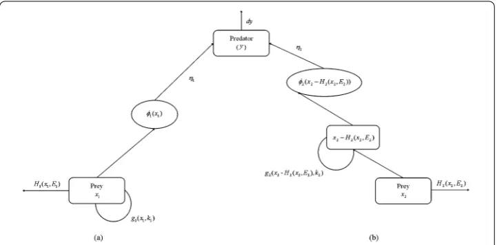
Xiao and Jennings [22] systematically studied the dynamical properties of the ratio-dependent predator–prey model with nonzero constant harvesting. They have shown that the harvested system can exhibit far richer dynamics compared to the model with no har-vesting, such as numerous kinds of bifurcations. Das et al. [19] considered a simple two species predator–prey model in which both species are harvested in proportion. The dy-namical behavior of the exploited system has been examined and the optimal harvesting policy has been studied. Li et al. [21] considered a bioeconomic predator–prey model with Holling type II functional response and nonlinear prey harvesting. The effect of economic profit on the proposed model has been analyzed by viewing it as a bifurcation parameter. In these traditional harvested predator–prey models, the harvesting function appears as a separate item. Human’s harvesting and the internal reproduction of a biological system itself take place simultaneously. The change in prey population density is indicated directly as the difference value between the number of growth and the number of prey captured by predator and human. Considering the impact of harvesting on the system, we propose that the changes in population density next time should not include the part harvested by the human. We are likely to overlook the point that the part harvested by the human no longer affects the reproduction of the species group; in other words, the part harvested by the human has no concern with the whole, and they can not be captured by predator species again. The relevant schematic is presented in Figure1.

Some authors considered a prey–predator system with a proportion refuge [23–26]. Lv et al. [23] studied the model incorporating a refuge protectingm1xof the prey, wherem1

(m1∈[0, 1]) is a constant, which leaves (1 –m1)xof the prey available to the predator.

Ma et al. [26] proposed a patchy predator–prey model with one patch as refuge and the other as open habitat and incorporated prey refugexRin the considered model explicitly.

Figure 1The sketch map of the two forms of harvesting functions. (a) A harvested predator–prey model with traditional form of harvesting function. (b) A harvested predator–prey model with a new form of harvesting function, whereφ1andφ2denote the predator response function of two prey species, respectively.η1and

η2are the rate of conversion of prey.g1andg2are the growth pattern of two prey species.mis the per capita

death rate of predator

teams of prey interacting with one team of predators and the harvesting function for two prey species takes different forms:

⎧ ⎪ ⎪ ⎪ ⎪ ⎪ ⎨ ⎪ ⎪ ⎪ ⎪ ⎪ ⎩

dx1

dt =x1g1(x1,k1) –yφ1(x1) –H1(x1,E1) –σ(x1,x2–H2(x2,E2)), dx2

dt = (x2–H2(x2,E2))g2(x2–H2(x2,E2),k2) –yφ2(x2–H2(x2,E2))

–σ(x1,x2–H2(x2,E2)), dy

dt =η1φ1(x1)y+η2φ2(x2–H2(x2,E2))y–my.

(1.3)

In this model, the harvesting function for the first preyx1adopts the traditional form and

the other harvesting function for the second preyx2takes the new form we proposed, in

which the number of species at the next moment is the change of the part which is not harvested by humans. Further, the harvesting of the prey also affects the growth of the predator in that the prey harvested by humans can not be captured by predator again.σ represents interspecific competition between the two prey species. Researching the dy-namics of predator–prey system (1.3) is the focus of this paper. And this kind of model is analyzed in detail through a concrete example.

This paper is organized as follows. The mathematical model is formulated in Sect.2. In Sect.3, for underlining the importance of the two different systems before combining the two harvesting forms into one model, we make a brief analysis of the dynamics of the two subsystems, in which preyx1orx2does not exist. The analyses of positivity and

sys-tem, and making a more in-depth comparison and analysis between the two harvesting functions. Discussion and concluding remarks are presented in Sect.8.

2 Mathematical model

In this paper, in order to draw a precise comparison, based on the model presented in [27], we make two prey species have the same growth function and functional response of the predator, in addition, consider the two-prey one-predator system with proportionate harvesting, then (1.3) takes the form

⎧ ⎪ ⎪ ⎪ ⎪ ⎪ ⎪ ⎪ ⎪ ⎨ ⎪ ⎪ ⎪ ⎪ ⎪ ⎪ ⎪ ⎪ ⎩

dx1

dt =r1x1(1 – x1

k1) –β1x1y–q1E1x1–σx1(x2–q2E2x2)

x1f1(x1,x2,y,E1,E2), dx2

dt =r2(x2–q2E2x2)(1 –

x2–q2E2x2

k2 ) –β2(x2–q2E2x2)y –σx1(x2–q2E2x2)(1 –q2E2)x2f2(x1,x2,y,E2), dy

dt =η1β1x1y+η2β2(x2–q2E2x2)y–myyg(x1,x2,E2),

(2.1)

here

⎧ ⎪ ⎪ ⎨ ⎪ ⎪ ⎩

f1(x1,x2,y,E1,E2) =r1(1 –_kx1₁) –β1y–q1E1–σx2(1 –q2E2), f2(x1,x2,y,E2) =r2[1 –(1–q_k2₂E2)x2] –β2y–σx1,

g(x1,x2,E2) =η1β1x1+η2β2(1 –q2E2)x2–m.

(2.2)

The following assumptions are taken into account for system (2.1):

1. Assume that the three species are subject to the positive initial conditions. 2. The growth pattern of two prey species is simulated with logistic equation in the

absence of predator and harvesting, of which the parameterrirepresents the

intrinsic growth rate of preyxi(i= 1, 2),kiis the carrying capacity of preyxi.

3. dis the per capita death rate of the predatory.

4. For simplicity, the feeding rate of the predator species is assumed to increase linearly with prey density [18,27]. The predator captures preyxi(i= 1, 2) at a rate

proportional to prey abundance with rate coefficientβi, and this contributes to an

increase in the predator population with a conversion rate ofηi[28]. Sinceηi= 1

represents a biomass of foraged prey can be completely converted to predator without any loss [29,30], which could not possibly happen in real life. Therefore we assumed0 <η1< 1and0 <η2< 1[31] in this paper.

5. The constantEiis the harvesting effort of preyxi(i= 1, 2).qiis the catchability

coefficient of preyxi. It is biologically meaningful to consider the case when

1 –q2E2> 0. Further, the predator population is not harvested.

6. ri,ki,βi,ηi,σ,mare positive rate constants.

3 The analysis of two subsystems

3.1 In the absence of preyx2

Model (2.1) in the absence of preyx2is equivalent to the predator–prey model with

tra-ditional harvesting function given by

⎧ ⎨ ⎩

dx1

dt =r1x1(1 – x1

k1) –β1x1y–q1E1x1,

dy

dt =η1β1x1y–my,

(3.1)

subject to the positive initial conditionsx1(0) > 0,y(0) > 0.

System (3.1) has a unique interior equilibrium pointS∗₁(x˜1,y˜) where

˜

x1= m η1β1

, y˜= 1 β1

r1

1 – d η1β1k1

–q1E1 . (3.2)

We can easily prove thatS₁∗(x˜1,y˜) is locally as well as globally stable ifE1<_qr1₁(1 –β1ηm1k1), which is the condition of its existence.

3.2 In the absence of preyx1

Model (2.1) in the absence of preyx1is equivalent to the predator–prey model with a new

form harvesting function given by

⎧ ⎨ ⎩

dx2

dt =r2(1 –q2E2)x2[1 –

(1–q2E2)x2

k2 ] –β2(1 –q2E2)x2y,

dy

dt =η2β2(1 –q2E2)x2y–my

(3.3)

subject to the positive initial conditionsx2(0) > 0,y(0) > 0.

System (3.3) has a unique interior equilibrium pointS∗₂(x¯2,y¯) where

¯

x2=

m η2β2(1 –q2E2)

, y¯= r2 β2

1 – m η2β2k2

. (3.4)

Similarly,S∗₂(x¯2,¯y) is locally as well as globally stable ifm<η2β2k2andE2< 1/q2, which

are also the conditions of its existence. Further, after rearranging the form of differential equation (3.3), system (3.3) becomes of the following form:

⎧ ⎨ ⎩

dx2

dt =r2x2(1 – x2

k2) –β2x2y–δ1(x2,y,E2),

dy

dt =η2β2x2y–my–δ2(x2,y,E2),

(3.5)

where

δ1(x2,y,E2) =q2E2x2

r2

1 –2x2–q2E2x2 k2

–β2y ,

δ2(x2,y,E2) =η2β2q2E2x2y.

Compared with the form of model (3.1), the termsδ1andδ2may be the correction terms

In addition, observing the composition of the two interior equilibrium points

S∗₁(x˜1,y˜) =

m η1β1

, 1 β1

r1

1 – m η1β1k1

–q1E1 ,

S∗₂(x¯2,y¯) =

m η2β2(1 –q2E2)

, r2 β2

1 – m η2β2k2

,

we know that onlyx¯2has connection with the harvesting effortE2in the form ofS∗2. The

opposite situation occurs inS₁∗. As human harvesting is considered, the harvesting value Eimay influence the quantity of preyxi(i= 1, 2) in equilibrium point directly, then the

form ofS∗₂is easier to be understood than the form ofS∗₁in biological terms. The further comparison and analysis of two forms of harvesting functions are carried out by numerical simulation in Sect.7.

4 Positivity and boundedness of the solutions

In this section, we study the positivity and boundedness of the solutions of system (2.1).

Theorem 1 All the solutions of system(2.1)with the positive initial conditions are positive for all t≥0and uniformly bounded.

Proof From system (2.1) with positive initial conditions, we have

x1(t) =x1(0)exp

t

0

r1x1(s)

1 –x1(s) k1

–β1x1(s)y(s) –s1x1(s) –σs2x1(s)x2(s) ds

> 0,

x2(t) =x2(0)exp

t

0

r2s2x2(s)

1 –s2x2(s) k2

–β2s2x2(s)y(s) –σs2x1(s)x2(s) ds

> 0,

y(t) =y(0)exp

t

0

η1β1x1(s)y(s) +η2β2s2x2(s)y(s) –my(s)

ds

> 0,

wheres1=q1E1,s2= 1 –q2E2.

Now, we define the functionΩ(t) =η1x1+η2x2+y.

Then differentiatingΩwith respect totand using the equations in system (2.1), we have

dΩ(t) dt =η1

dx1 dt +η2

dx2 dt +

dy dt

=η1r1x1(1 –x1/k1) –η1s1x1– (η1+η2)σs2x1x2+η2r2s2x2(1 –s2x2/k2) –my.

Therefore,

dΩ

dt +mΩ= – η1r1

k1

x1–

k1(r1–s1+m)

2r1 2

+k1η1(r1–s1+m)

2

4r1

–η2r2s

2 2 k2

x2–

k2(r2s2+m)

2r2s22 2

+k2η2(r2s2+m)

2

4r2s22

≤k1η1(r1–s1+m)2

4r1

+k2η2(r2s2+m)

2

4r2s22

L> 0.

The right-hand side of the above inequality is bounded for (x1,x2,y)∈R3+.

Applying the theory of differential inequality, we have

0 <Ω(t)≤ L m

1 –e–mt_+Ω(0)e–mt_{. (4.1)}

Ast→ ∞, we can see that the limit of the right-hand side of (4.1) isL/m. Hence, by the definition ofΩ(t), we can imply that all the solutions of system (2.1) are bounded in the interior ofR3

+.

The proof is complete.

5 Existence and stability of equilibria

In this section we investigate the existence and stability of the equilibrium points of system (2.1) in the closed first quadrant.

5.1 Existence of equilibria

Model system (2.1) possesses seven equilibrium points including one trivial, two axial, three boundary, and one interior equilibrium point.

1. The trivial equilibrium pointS0= (0, 0, 0)exists irrespective of any parametric

restriction.

2. Two axial equilibrium points of model (2.1) are given byS1(0,xˆ2, 0)andS2(x˘1, 0, 0),

where

ˆ

x2= k2

1 –q2E2

, x˘1=k1

1 –q1E1 r1

. (5.1)

Clearly,S1exists when the assumptionE2< 1/q2holds, the feasibility condition for S2isE1<r1/q1, which isE1< BTPx1. The ratio (r1/q1) of the biotic potential to the catchability coefficient (q1) is known as the biotechnical productivity (BTP) of prey x1species [32].

3. In the absence of preyx1the boundary equilibrium point in thex2y-plane is given

byS3(0,x¯2,y¯), wherex¯2andy¯are given in (3.4). The feasible condition forS3is m<η2β2k2.

4. In the absence of preyx2the boundary equilibrium point in thex1y-plane is given

byS4(x˜1, 0,y˜), wherex˜1andy˜are given in (3.2). The feasible condition forS4is E1<_qr1₁(1 –η1βm1k1).

5. The predator-free boundary equilibrium point in thex1x2-plane is given by S5(xˇ1,xˇ2, 0), where

ˇ

x1=

r2k1(k2σ+q1E1–r1)

σ2_k

1k2–r1r2

, xˇ2=

r1(k1–xˇ1) –q1E1k1

σk1(1 –q2E2)

. (5.2)

The feasible existence ofS5demands the parametric restriction

(k2σ+q1E1–r1)

σ2k1k2–r1r2

6. Apart from the axial and boundary equilibrium points, there is a unique interior equilibrium pointS∗(x∗₁,x∗₂,y∗)with

x∗₁=mv2+η2β2[–r2β1+β2(r1–q1E1)] η2β2v1+η1β1v2

, x∗₂= m–η1β1x ∗

1

η2β2(1 –q2E2)

,

y∗= 1 β1

r1

1 –x ∗

1 k1

–q1E1–σx∗2(1 –q2E2) ,

(5.4)

wherev1=β2_k1r1 –σβ1,v2=β_k1₂r2–σβ2.

The interior equilibrium point is feasible when each term ofS∗(x∗₁,x∗₂,y∗)is greater than zero. Due to the complexity of the calculation, we carry out detailed analysis in Sect.7.2.

5.2 Local stability of equilibria

Here we provide the local stability conditions for feasible equilibrium points of system (2.1) based on the standard linearization technique, and then use the famous Routh– Hurwitz criterion [33] to determine the properties of eigenvalues of the matrix associ-ated with the linearized version. Ify= 0, system (2.1) becomes a two-species competitive model, in which we are not interested. In this section, we mainly study the following steady states:S0(0, 0, 0),S3(0,x¯2,¯y),S4(x˜1, 0,y˜), andS∗(x1∗,x∗2,y∗).

The Jacobian matrix of system (2.1) at any point (x1,x2,y) takes the form

J(x1,x2,y)=

⎡ ⎢ ⎣

ζ11 ζ12 ζ13

ζ21 ζ22 ζ23

ζ31 ζ32 ζ33

⎤ ⎥

⎦, (5.5)

where

ζ11= –q1E1–β1y–r1

2x1 k1

– 1

–σ(1 –q2E2)x2, ζ12= –σx1(1 –q2E2),

ζ13= –β1x1, ζ21= –σx2(1 –q2E2), ζ23= –β2x2(1 –q2E2),

ζ22= –(1 –q2E2)

2r2x2(1 –q2E2) k2

+β2y+σx1–r2 ,

ζ31=β1η1y, ζ32=β2η2y(1 –q2E2), ζ33=β1η1x1–m+β2η2(1 –q2E2)x2.

5.2.1 Stability of S0= (0, 0, 0)

The eigenvalues of the JacobianJ(S0) evaluated at the trivial equilibrium pointS0= (0, 0, 0)

areλ1=r1–q1E1,λ2=r2(1 –q2E2) > 0, andλ3= –m< 0. HenceS0is a saddle point with

dimWs(S0) = 2 anddimWu(S0) = 1 if condition (I)E1> BTPx1is satisfied andS0is a saddle point withdimWs_(S

0) = 1 anddimWu(S0) = 2 if condition (I) is violated, wheredimWs

anddimWu_{denote the dimensions of stable and unstable subspaces, respectively.}

5.2.2 Stability of S3= (0,x¯2,y¯)

One of the eigenvalues ofJ(S3) is given by

¯

λ1=r1–q1E1+

β1r2(m–β2η2k2)

β₂2η2k2

– mσ β2η2

and the other eigenvaluesλ¯_±are determined by the quadratic equation (see Appendix1). Based on the existence condition ofS3, we have

Tr[J¯S3] =

mr2(q2E2– 1)

β2η2k2

< 0, λ¯+λ¯–=Det

mr2(m–β2η2k2)(q2E2– 1)

η2β2k2

> 0.

Then we haveS3is locally asymptotically stable if the condition

(II) E1>

1 q1

r1+

β1r2(m–β2η2k2)

β₂2η2k2

– mσ β2η2

(=E¯1)

is satisfied. Otherwise,S3is a saddle point withdimWs(S3) = 2 anddimWu(S3) = 1.

Eco-logically, we can say that in this case the coexistence of preyx2and the predator is possible

if the harvesting effort of preyx1exceeds the critical valueE¯1.

5.2.3 Stability of S4= (x˜1, 0,y˜)

The characteristic equation for the variational matrixJ(S4) isλ3+ϕ1λ2+ϕ2λ+ϕ3= 0 (see

Appendix2).

According to the Routh–Hurwitz criterion,S4is locally asymptotically stable ifϕ1> 0,

ϕ3> 0, andϕ1ϕ2–ϕ3> 0.

5.2.4 Stability of S∗= (x∗₁,x∗₂,y∗)

The characteristic equation associated with the matrixJ(S∗) is given byλ3+ξ1λ2+ξ2λ+

ξ3= 0 (see Appendix3).

According to the Routh–Hurwitz criterion, the interior equilibrium pointS∗ is locally asymptotically stable ifξ1> 0,ξ3> 0, andξ1ξ2–ξ3> 0. It is quite difficult to find explicit

parametric restriction for the local asymptotic stability ofS∗, so we discuss it for some specific choice of system parameters in Sect.7.2.

5.3 Global stability analysis

In this section, we consider the global asymptotic stability for the interior equilibrium pointS∗with the help of Lyapunov functional construction method [34].

Theorem 2 The positive interior equilibrium point S∗(x∗₁,x∗₂,y∗)is globally asymptotically stable if4η1η2r1r2>σ2k1k2.

Proof Obviously, (x∗₁,x∗₂,y∗) satisfies the equalities

⎧ ⎪ ⎪ ⎨ ⎪ ⎪ ⎩

r1(1 –x ∗

1

k1) –β1y ∗_–q

1E1–σx∗2(1 –q2E2) = 0, r2[1 –

(1–q2E2)x∗2

k2 ] –β2y ∗_–σx∗

1= 0,

η1β1x∗1+η2β2(1 –q2E2)x∗2–m= 0,

(5.6)

which are equivalent to

⎧ ⎪ ⎪ ⎨ ⎪ ⎪ ⎩

r1=q1E1+β1y∗+_kr1₁x∗1+σx∗2(1 –q2E2), r2=β2y∗+r_k2₂(1 –q2E2)x∗2+σx∗1, m=η1β1x∗1+η2β2(1 –q2E2)x∗2.

Now we show the global stability of interior equilibrium pointS∗by constructing the Lya-punov function [35],V(x1,x2,y) :R3+→R, s.t.

V(x1,x2,y) =V1(x1,x2,y) +V2(x1,x2,y) +V3(x1,x2,y), (5.8)

whereV1(x1,x2,y) =η1(x1–x∗1–x∗1lnxx1∗₁),V2(x1,x2,y) =η2(x2–x∗2–x∗2lnxx2∗₂),V3(x1,x2,y) =

y–y∗–y∗ln_yy∗.

From (5.8), we have

∂V(x1,x2,y)

∂xi

=ηi

1 –x ∗

i

xi

(i= 1, 2), ∂V(x1,x2,y) ∂y = 1 –

y∗

y, (5.9)

which shows that the positive equilibrium (x∗₁,x∗₂,y∗) is the only extremum of the function V(x1,x2,y) in the positive quadrant [36]. Then we can easily verify that

lim x1→0

V(x1,x2,y) = lim x2→0

V(x1,x2,y) =lim

y→0V(x1,x2,y) = +∞,

lim x1→+∞

V(x1,x2,y) = lim x2→+∞

V(x1,x2,y) = lim

y→+∞V(x1,x2,y) = +∞.

(5.10)

Combining (5.9) and (5.10), we observe that the positive equilibrium is the global min-imum. Further, it can be verified that the functionV(x1,x2,y) is zero at (x∗1,x∗2,y∗). Then

we haveV(x1,x2,y) >V(x∗1,x∗2,y∗) = 0 for allx1,x2,y> 0.

The time derivative ofV1along the solution of (2.1) is

dV1 dt =η1

x1–x∗1

r1

1 –x1 k1

–β1y–q1E1–σx2(1 –q2E2) . (5.11)

After some simplifications and with the help of the first equation of (5.7), (5.11) takes the following form:

dV1 dt = –

η1r1 k1

x1–x∗1

2

–η1β1

x1–x∗1

y–y∗

–σ η1(1 –q2E2)

x1–x∗1

x2–x∗2

.

Similarly, we have

dV2 dt = –

η2r2(1 –q2E2)2(x2–x∗2)2 k2

–η2β2(1 –q2E2)

x2–x∗2

y–y∗

–σ η2(1 –q2E2)

x1–x∗1

x2–x∗2

,

dV3 dt =η1β1

x1–x∗1

y–y∗+η2β2(1 –q2E2)

x2–x∗2

Then taking the time derivative ofV(x1,x2,y) along the trajectories of (2.1), after proper

simplification [35], we have

dV(x1,x2,y)

dt = dV1 dt + dV2 dt + dV3 dt

= –η1r1 k1

x1–x∗1

2

–η1β1

x1–x∗1

y–y∗

–σ η1(1 –q2E2)

x1–x∗1

x2–x∗2

–η2r2 k2

(1 –q2E2)2

x2–x∗2

2

–η2β2(1 –q2E2)

x2–x∗2

y–y∗

–σ η2(1 –q2E2)

x1–x∗1

x2–x∗2

+η1β1

x1–x∗1

y–y∗

+η2β2(1 –q2E2)

x2–x∗2

y–y∗

= –

η1r1 k1

x1–x∗1

2

+η2r2 k2

(1 –q2E2)2

x2–x∗2

2

+σ(η1+η2)(1 –q2E2)

x1–x∗1

x2–x∗2

= –XTAX,

whereX= [(x1–x∗1), (x2–x∗2)]Tand

A=

_η

1r1

k1

σ

2(η1+η2)(1 –q2E2) σ

2(η1+η2)(1 –q2E2)

η2r2

k2 (1 –q2E2)

2

.

ThereforedV/dt< 0 ifAis positive definite. TheAis positive definite if the hypothesis of

Theorem2is satisfied.

From the above analysis, we can see that the interior equilibrium is globally asymp-totically stable under certain conditions. If the system is stable prior to harvesting, the harvested system does not change its stability.

6 The yield problem of system (2.1)

When it comes to biological conservation, there are many tools to do this. For exam-ple, the maximum sustainable yield (MSY) policy [37], the optimal taxation policy [38], the marine protected areas [7], the impulsive harvesting [39], and so on. As we all know, the maximum sustainable yield policy is a classic and old strategy. Despite it has many shortcomings [40], the concept of MSY has been a central theme for fisheries and legally adopted by Johannesburg Implementation Plan, for world fisheries to catch a maximum that is sustainable and to supposedly preserve over-fished stocks [41]. Ghosh et al. [41] defined the total maximum sustainable yield (MSTY) as the maximum of the sum of the yields obtained from both prey and predator under independent harvesting efforts. The MSTY is obtained when the yield is maximized with respect toE1andE2. In this section,

we investigate the maximum yield of system (2.1) and explore whether the system has MSTY.

system (3.3) isY(E2) =q2E2x¯2=η2β2(1/mq2E2–1). Further,Y _(E

2) = _η mq2

2β2(1–q2E2)2 > 0. We can see that the yieldY(Ei) (i= 1, 2) increases with the increase of harvesting effortEi(i= 1, 2).

Hence, there is no MSY in either of two subsystems. In system (2.1), we have

Y(E1,E2) =q1E1x∗1+q2E2x∗2

=q1E1(v3–η2β

2 2q1E1) v4

+q2E2(v5+v6E1) 1 –q2E2

= –q

2 1η2β22

v4 E2₁+

q1v3 v4

+ v6q2E2 1 –q2E2

E1+ v5q2E2

1 –q2E2

, (6.1)

wherev3=mv2–η2β2r2β1+η2β22r1,v4=η2β2v1+η1β1v2,v5=v4m_v4–_ηη₂1_ββ₂1v3,v6=

η1β1η2β₂2q1 η2β2v4 . The Hessian matrix corresponding toYis

H=

⎡ ⎣–

2β₂2η2q21

v4

q2v6

(q2E2–1)2

q2v6

(q2E2–1)2 –

2q22(v5+E1v6)

(q2E2–1)3

⎤

⎦. (6.2)

Obviously1= – 2β₂2η2q12

v4 < 0 ifv4> 0; meanwhile,

2= –

q2₂[v2v26+ 4β22η2q21(1 –q2E2)(v5+E1v6)] v4(1 –q2E2)4

= –β

2

1β22η12q21q22 v2₄(1 –q2E2)4

< 0.

For the existence of maximum ofYat (E∗₁,E∗₂), the sufficient conditions are not satisfied. If we fix the parameterE2, letYreach its maximum atEM1 =

v3q1(1–q2E2)+q2E2v6v4

2η2β₂2q21(1–q2E2) forv4> 0.

Then substitutingEM

1 into (6.1), we have

Y(E) = v4v

2 6

4β₂2η2q21

E2+2v5β

2

2η2q1+v3v6

2β₂2η2q1

E+ v

2 3

4v4β22η2

, (6.3)

whereE= q2E2

1–q2E2.

We find thatY(E) is a quadratic function ofEgoing upwards forv4> 0.Y(E) can not

get maximum in the feasible region aboutE2. Functions in (6.1) and (6.3) can not take the

maximum at the same time. We will give a concrete example to explain the problem in detail in Sect.7.3.

Since there is no MSTY in system (2.1), we establish a control problem for yield to find a suboptimal control strategy. The form of objective functionGis expressed as follows:

G(E1,E2) =

tf

0

(q1E1x1+q2E2x2)dt, (6.4)

which is subjected to the state equation (2.1) and the control variablesEi(t) are subjected

to

U=E1(t),E2(t)

∈L1[0,tf]×L1[0,tf]|a1≤E1(t)≤b1,a2≤E2(t)≤b2

,

where ai, bi (i= 1, 2) are fixed normal quantities. The initial condition is (x1(0),x2(0), y(0)) = (x10,x20,y0). To ensure the sustainable survival of the species, we set the state

ca-pacity of preyxi(i= 1, 2). We hope to get the maximum yield in [0,tf], which is equivalent

to minimizing –G. The optimal control problem (P) is as follows:

min E1(t),E2(t)∈U–G

E1(t),E2(t)

,

dx1

dt =x1f1(x1,x2,y,E1,E2), x1(0) =x10, dx2

dt = (1 –q2E2)x2f2(x1,x2,y,E2), x2(0) =x20, dy

dt =yg(x1,x2,E2), y(0) =y0,

0 <x1(t) <k1, 0 <x2(t) <k2, y(t) > 0, ∀t∈[0,tf].

(6.5)

We use the computational algorithms based on the concept of control parametrization to solve the optimal control problem. First, we partition the interval [0,tf] into several

subintervals, and the control variables Ei (i= 1, 2) are approximated by piecewise

con-stant functions with the incon-stants of switching preassigned by the corresponding partition. Then, an optimal control problem is approximated by a corresponding optimal parame-ter selection problem which can be viewed as a mathematical programming problem, and hence is solvable by the existing optimization software packages [42, 43]. The relevant numerical experiment is shown in Sect.7.3.

7 Numerical simulations

In this section, to make analytical studies more complete, we perform numerical simula-tions by MATLAB. The numerical simulasimula-tions of systems (2.1), (3.1), and (3.3) have been carried out from the following four aspects.

7.1 The role of the carrying capacity of preyxi(i= 1, 2)

The term carrying capacity was put forward by Leopold in his work [44] and is one of the most common concepts in wildlife management [45]. Many types of research [46,47] have verified that carrying capacity makes a great difference in the predator–prey system. Next, we use numerical simulations to investigate the impact of carrying capacityki(i= 1, 2)

on the system result. We selectk1andk2 from three levels and the order of magnitude

between them is 10. The other parameter values are as follows. The time graph and path of model (2.1) aski(i= 1, 2) is changing with different orders of magnitude are given in

Figure2.

r1= 2.09, β1= 0.01, q1= 0.04, η1= 0.3, σ= 0.001,

r2= 2.07, β2= 0.02, q2= 0.01, η2= 0.3, m= 0.05.

(7.1)

By simple calculation and observation, we can obtain that if we just change the magnitude ofki(i= 1, 2), the time for the system to reach equilibrium also increases exponentially (see

Figure2), and the range ofE1used to make three species coexistence (S∗) is also reduced

when keeping the other parameters unchanged andE2< 1/q2. When the carrying capacity ki(i= 1, 2) is very large, the growth of prey species tends to increase exponentially, which

is not realistic. Therefore, we choose suitable medium size values of ki(i= 1, 2) in the

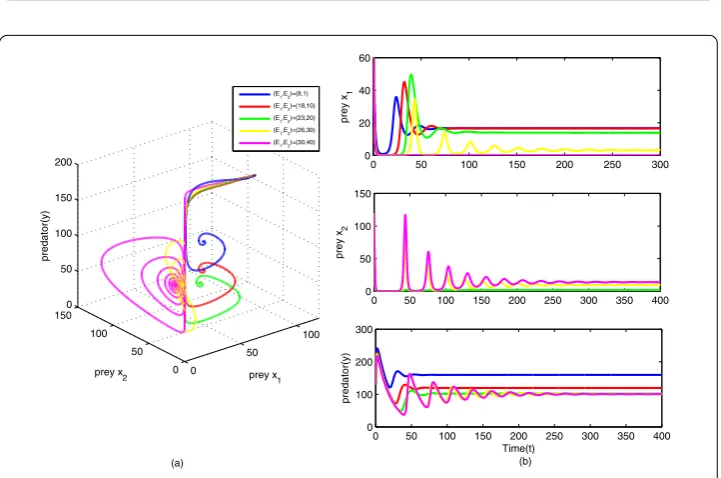
Figure 2Phase portrait and time graph of model (2.1) around the interior equilibrium point. (a), (b)k1= 20,

k2= 30. (c), (d)k1= 200,k2= 300. (e), (f)k1= 2000,k2= 3000. (E1,E2) = (26.2, 45). The other parameter values

are given in (7.1)

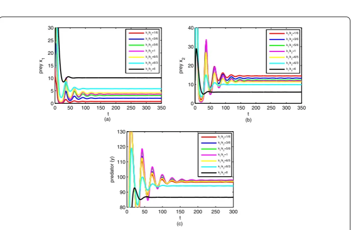
Figure 3The changes of the biomass of system species withk1/k2. (a) Variations in preyx1with increasing

time. (b) Variations in preyx2with increasing time. (c) Variations in predator (y) with increasing time. The

parameter values are given in (7.1) and (E1,E2) = (26.2, 45)

Further, we change the ratio betweenk1 andk2 to investigate the dynamics of three

species using numerical simulation (see Figure3). Simulation results show that the time for the system to reach equilibrium state decreases with the increase of ratiok1/k2when k1/k2> 1. On the contrary, the time for the system to reach equilibrium state increases

7.2 The simulation about the model equations around three equilibrium points We simulate the model equations around various biologically significant steady states. In the previous analysis, we have identified two important boundary steady statesS3(0,x¯2,¯y)

(without preyx1) andS4(x˜1, 0,y˜) (without preyx2) together with the steady state of

coex-istenceS∗(x∗₁,x∗₂,y∗).

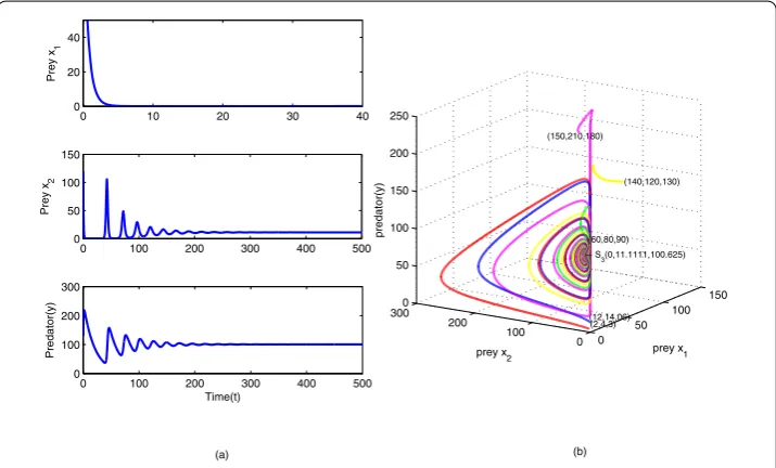
First, we calculate the two threshold harvesting efforts using the stability and existence conditions of three equilibrium points, then we select a stable state for each equilibrium point. The time evolution of the populations aroundS3 is shown in Figure4(a), which

shows that the predator coexists stably with the second prey instead of the first one and the first prey goes to extinction. We have also shown the phase portrait around this equi-librium point in Figure4(b). The time evolution of the populations aroundS4, which is

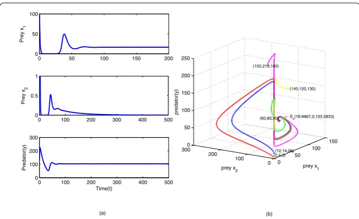
stable, is shown in Figure5(a) and the relevant phase portrait is shown in Figure5(b), which shows stable coexistence of the first prey and the predator.

Finally, we mainly consider the local dynamics of the unique interior equilibrium using numerical simulation. For better comparison, we take the following values:

r1=r2= 2, k1=k2= 200, β1=β2= 0.01,

q1=q2= 0.2, η1=η2= 0.4, σ= 0.008, m= 0.05.

(7.2)

The relevant functions are as follows:

⎧ ⎪ ⎪ ⎨ ⎪ ⎪ ⎩

f1(x1,x2,y,E1,E2) = 2(1 –₂₀₀x1) – 0.01y– 0.2E1– 0.008(1 – 0.2E2)x2,

f2(x1,x2,y,E2) = 2[1 –(1–0.2₂₀₀E2)x2] – 0.01y– 0.008x1,

g(x1,x2,E2) = 0.004x1+ 0.004(1 – 0.2E2)x2– 0.05.

(7.3)

Figure 4Numerical simulation of model (2.1) around the boundary stateS3.S3(0, 11.1111, 100.625) with

E1= 30,E2= 25. Different color curves represent different initial conditions. The other parameter values are

Figure 5Numerical simulation of model (2.1) around the boundary stateS4.S4(16.6667, 0, 103.5833) with

E1= 22,E2= 35. Different color curves represent different initial conditions. The other parameter values are

given in (7.1) and (k1,k2) = (200, 300)

The interior equilibrium is

S∗x∗₁,x∗₂,y∗=

6.25 – 50E1,

50E1+ 6.25

1 – 0.2E2

, 188.75 – 10E1

. (7.4)

The feasible condition forS∗is 0 <E1< 0.125 and 0 <E2< 5. Moreover, the characteristic

equation associated with the matrixJ(S∗) is given byλ3+ξ1λ2+ξ2λ+ξ3= 0, where

ξ1= 0.2890×10–16E1– 0.0125E2– 0.1E1E2+ 0.1250,

ξ2= 0.0220E21E2– 0.0097E2– 0.0750E1E2– 0.0050E1– 0.0900E21+ 0.0958,

ξ3= 0.0000125E1E2– 0.000236E2– 0.0000625E1+ 0.0151E12E2

– 0.0008E3

1E2– 0.0755E21+ 0.0040E31+ 0.0012.

Further, we have

ξ1ξ2–ξ3=

–0.0022E₁3+ 0.00722E2₁+ 0.0019E1+ 0.0001

E₂2

+0.0098E3₁– 0.0107E2₁– 0.0189E1– 0.0022

E2

– 0.004E3₁+ 0.0643E2₁– 0.0006E1+ 0.01079.

To investigate its stability, we examine the signs of functionsξ1,ξ2andξ1ξ2–ξ3.

1. Ifξ1> 0, we haveE2<0.2890×10

–16_E 1+0.125

0.0125+0.1E1 < 10, which is obviously true.

2. Ifξ3> 0, we haveφ(E2– 5) > 0, whereφ= –0.8E31+ 15.1E21+ 0.0125E1– 0.236.

Further,φ= –2.4E2

1+ 30.2E1+ 0.0125, the two roots of this equationφ= 0are

Figure 6Numerical simulation of model (2.1) around the interior equilibrium pointS∗.

S∗(2.25, 13.4868, 187.955) withE1= 0.08,E2= 1.2. Different color curves represent different initial conditions.

The other parameter values are given in (7.2)

3. Considerξ1ξ2–ξ3, let

φ1= –0.0022E31+ 0.00722E21+ 0.0019E1+ 0.0001,

φ2= 0.0098E31– 0.0107E21– 0.0189E1– 0.0022,

φ3= –0.004E13+ 0.0643E12– 0.0006E1+ 0.01079.

Thenξ1ξ2–ξ3=φ1E22+φ2E2+φ3. After computation, we haveφ1> 0and

=φ₂2– 4φ1φ3< 0whenE1belongs to(0, 0.125), therefore,ξ1ξ2–ξ3> 0.

From the above analysis, the unique interior equilibrium is locally asymptotically sta-ble. Next we simulate the model equations around the interior equilibrium pointS∗. The resulting time and phase plot are shown in Figure6.

7.3 Simulation for the yield problem of system (2.1)

Let us give a concrete example to analyze the yield problem of system (2.1). The relevant parameters, exceptm= 0.4,σ = 0.0035, are given in (7.1) and (k1,k2) = (200, 300). The

interior equilibrium is

121.2296 – 4.6110E1, –

0.0138E1+ 0.0363

0.00006E2– 0.006

, 0.0115E1+ 80.1969

.

The feasible condition is 0≤E1< 26.29139, 0≤E2< 100. Consider that the yield

func-tion has a maximum value of the parameterE1 when E2 is fixed. Then we have EM1 = 0.020833(331E2–63,100)

E2–100 andY(E) = 7.204611E

2_{–36.359270E+31.873279. The feasible region of}

Eis 0 <E< 2.103333, whenE= 2.103333, namelyE2= 67.776584, we haveEM1 = 26.29139,

thenx∗₁= 0. Further,Y(E2= 0) = 31.8732789 andY(E2= 67.776584) = 140.222222. Since

Figure 7The changes of the biomass of system species and the yield. (a) Preyx1biomass varies withE1

andE2. (b) Preyx2biomass varies withE1andE2. (c) The predator biomass varies withE1andE2. (d) The yield

from both prey and predator as function ofE1andE2. The relevant parameters exceptd= 0.4,σ= 0.0035 are

given in (7.1) and (k1,k2) = (200, 300)

Table 1 The optimal control and states variables of (P)

Time Control 1 Control 2 State 1 State 2 State 3 0.0000 0.83430 0.00000 15.00000 15.00000 12.00000 1.8182 5.16684 1.37425 109.00304 128.58783 16.10776 3.6364 3.96670 0.88688 93.32653 125.22972 66.42204 5.4545 1.09206 1.92634 71.50602 37.75527 113.98322 7.2727 3.41622 0.00000 80.79575 13.47770 105.64105 9.0909 6.96972 0.00000 89.77432 8.50216 90.45973 10.9091 21.48043 0.00000 91.47356 8.84428 77.90937 12.7273 23.47555 1.99791 59.29581 16.42672 62.38116 14.5455 12.68776 54.89466 50.81738 43.53919 54.60362 16.3636 5.90543 90.59718 81.84325 72.67257 50.86236 18.1818 26.29119 87.90424 122.91470 81.59493 47.76096 20.0000 26.29119 87.90424 67.05375 97.18600 41.09602

Here we use the MISER 3 Optimal Control Toolbox of MATLAB to solve problem (6.5). The relevant parameters exceptm= 0.4,σ= 0.0035 are given in (7.1) and (k1,k2) =

(200, 300). According to the existence condition of interior equilibrium point, the range

of control parametersEi(i= 1, 2) is given as 0≤E1≤26.29139, 0≤E1≤99.9999. In fact,

the value range of parameterE2is [0, 100). To guarantee that model (2.1) is significant, the

condition 1 –q2E2= 0 should be satisfied. So we setb2to 99.9999. The initial condition

is (x1(0),x2(0),y(0)) = (15, 15, 12) andtf = 20. One possible optimal solution is shown in

Figure 8The optimal states and control of problem (P)

Figure 9Different solution plots asE1increases. Keeping the other parameters unchanged (see Table2)

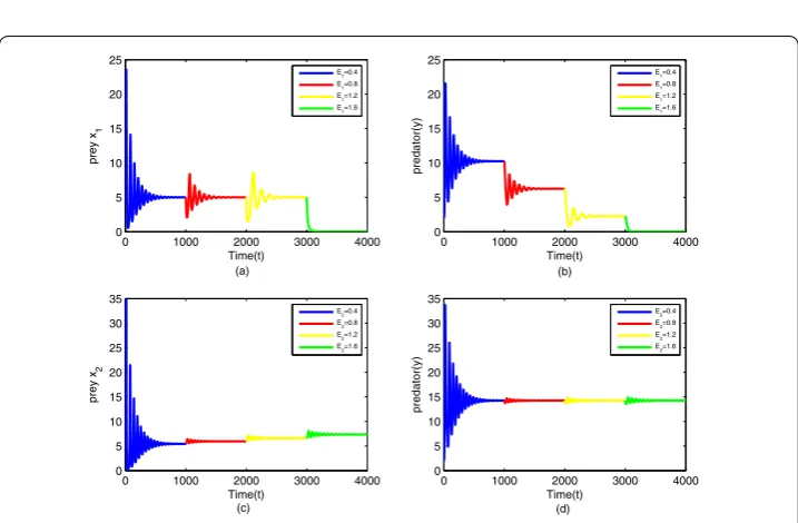
7.4 Influence of two forms of harvesting functions for systems (2.1), (3.1), and (3.3)

To compare the two forms of harvesting functions better, we perform the numerical sim-ulations of model (2.1) withE1andE2changing respectively (see Figures9,10,11). The

parameter values used in Figures9,10,11are given in Table2.

For subsystems (3.1) and (3.3), we keep the corresponding parameters exceptE1 and E2the same, then draw the time graphs and different solution plots of models (3.1) and

(3.3), respectively, asEi (i= 1, 2) increase (see Table3) (see Figure12). In addition, we

Figure 10 Different solution plots asE2increases. Keeping the other parameters unchanged (see Table2)

Figure 11 Different solution plots as bothE1andE2increase. See Table2

week period, then observe the population dynamic (see Figure13). We take the relevant parameters exceptE1andE2as follows:

r1=r2= 0.3, k1=k2= 100, β1=β2= 0.02,

q1=q2= 0.2, η1=η2= 0.5, m= 0.05.

(7.5)

From Figures9,10,11, by controlling the two harvesting effortsE1andE2, we can

dis-cover that if we just change the parameterE1, the number of three species in the final state

Table 2 The parameter values ofE1andE2used in Figures9,10,11

No. Fixed parameters (E1,E2) S∗(x∗1,x∗2,y∗) Figure

1 k1= 200,k2= 300,

ri,βi,qi,ηi,σandm are the same as (7.1)

(8, 45) Not exist Figure9(blue)

2 . . . (18, 45) Not exist Figure9(red) 3 . . . (23, 45) (13.9075, 2.5083, 102.3287) Figure9(green) 4 . . . (26, 45) (3.1693, 12.2704, 101.0132) Figure9(yellow) 5 . . . (30, 45) Not exist Figure9(magenta) 6 . . . (24, 1) (10.3281, 3.2013, 101.8902) Figure10(blue) 7 . . . (24, 10) (10.3281, 3.5214, 101.8902) Figure10(red) 8 . . . (24, 20) (10.3281, 3.9616, 101.8902) Figure10(green) 9 . . . (24, 30) (10.3281, 4.5275, 101.8902) Figure10(yellow) 10 . . . (24, 40) (10.3281, 5.2821, 101.8902) Figure10(magenta) 11 . . . (8, 1) Not exist Figure11(blue) 12 . . . (18, 10) Not exist Figure11(red) 13 . . . (23, 20) (13.9075, 1.7245, 102.3287) Figure11(green) 14 . . . (26, 30) (3.1693, 9.6410, 101.0132) Figure11(yellow) 15 . . . (30, 40) Not exist Figure11(magenta)

Table 3 The parameter values ofE1andE2used in Figure12

Ei(i= 1, 2) S∗1of (3.1) Figure S∗2of (3.3) Figure

0.4 (5, 10.25) Figure12(a)(b)(blue) (5.4348, 14.25) Figure12(c)(d)(blue) 0.8 (5, 6.25) Figure12(a)(b)(red) (5.9524, 14.25) Figure12(c)(d)(red) 1.2 (5, 2.25) Figure12(a)(b)(yellow) (6.5789, 14.25) Figure12(c)(d)(yellow) 1.6 Not exist Figure12(a)(b)(green) (7.3529, 14.25) Figure12(c)(d)(green) 2 Not exist Figure12(a)(b)(magenta) (8.3333, 14.25) Figure12(c)(d)(magenta)

system (2.1) is tiny except for preyx2species if we only changeE2. Further, from Figure12,

comparing with the coexistence stateS₁∗andS∗₂, as the intensity of capturing increases, the amount of preyx1remains unchanged finally, and the amount of the relevant predator

de-creases in system (3.1), while for system (3.3), the opposite is the case. The amount of prey x2increases and the amount of the relevant predator stays the same when the system turns

to be stable finally.

From Figure13, we can find that, for system (3.1), when the amount of harvesting ef-fort is changed regularly based on the previous level of the population, the ecosystem will produce large fluctuations and even the risk of extinction exists. However, as for system (3.3), when the system tends to balance the appropriate change in the amount of harvest-ing effort, the system will produce a small range of fluctuations, and finally tend to bal-ance, which is consistent with the global asymptotic stability of the internal equilibrium point and more in line with the development law of the real ecosystem. When the system achieves a stable equilibrium state of coexistence, increasing or decreasing harvesting will not easily break the balance of the system in that the ecosystem has the ability to repair itself.

Through the above analysis, we draw an interesting conclusion: the growth level of the predator–prey system under the effect of the new form of harvesting function is better than that under the impact of the traditional form, which may be a better reflection of the role of human-made disturbance in the development of a biological system. Under the same condition, the effect ofE2 on predation system (2.1) is more significant than that

ofE1. Combined with the analysis of maximum yield (Sect.6), harvesting may allow the

Figure 12 Path of the system species asE1(E2) increases. (a), (b) Path of prey speciesx1and predator species

yof system (3.1) asE1increases (see Table3) keeping the other parameters unchanged. (c), (d) Path of prey

speciesx2and predator speciesyof system (3.3) asE2increases (see Table3) keeping the other parameters

unchanged

Figure 13 Path of the system species asE1(E2) increases periodically. (a), (b) Path of prey speciesx1and

predator speciesyasE1increases periodically. The other parameter values are given in (7.5). (c), (d) Path of

prey speciesx2and predator speciesyasE2increases periodically. The other parameter values are given in

(7.5)

8 Discussion and concluding remarks

This paper has been conducting thorough research on the two-prey one-predator system, in which the harvesting function for prey x1adopts the traditional form and the other

harvesting function for preyx2takes the new form. For drawing a precise comparison, we

make two prey species have the same kind of growth function and functional response of the predator.

We focus on the stability of system (2.1). It has been proved that the positive interior equilibrium solutionS∗(x∗₁,x∗₂,y∗) is globally asymptotically stable under certain condi-tions (Theorem2). Further, from the comparison between two subsystems (3.1) and (3.3), we find that the new form of harvesting function refines the effects of human intervention, which shows that harvesting prey affects not only the growth of prey population but also the growth of predator population.

To obtain the complete analytical studies, we apply numerical simulations to verify the results from four aspects: investigating the role of the carrying capacity of prey (see Sect.7.1), simulating the model equations around four equilibrium points (see Sect.7.2), investigating the problem of maximum sustainable yield and dynamic optimal yield in finite time (see Sect.6and7.3), and studying the influence of two forms of harvesting functions for systems (2.1), (3.1), and (3.3) (see Sect.7.4). Through the method of con-trolling variables, on the one hand, the dynamic behavior of system (2.1) is analyzed; on the other hand, the effects of two forms of harvesting function on systems (2.1), (3.1), and (3.3) are studied. Taking the specific parameters of the two prey species to the same value, we investigate the existence and stability of interior equilibrium under the influence of two kinds of harvesting functions. Comparing systems (3.1) and (3.3), though the new model system shows similar dynamical behaviors as the traditional model in which the harvesting function appears as a separate item, the emphases of the two kinds of systems are different (see Figure1, in which process (a) emphasizes the effect of harvesting, while process (b) emphasizes the change of the system itself after harvesting). By analyzing the stability of the equilibrium points and the growth level of the predator–prey system, we find that the effect ofE2on predator system (2.1) is more significant than that ofE1. Under

the influence ofE1, the overall level of population number at which the system is stable

decreases as effort increases, but forE2, the opposite is the case.

If we regard human intervention as an incentive factor which may promote the growth level of the population, then the population at equilibrium will increase as shown in Ta-ble3and Figure12. Combined with the analysis of the yield problem, harvesting may allow the population to grow faster. Let us consider the fish as a single population which follows a simple logistic, and the population subject to the proportional harvesting. The maxi-mum sustainable yield is approached when the optimaxi-mum harvesting effort ofeopt=r/2

is applied, and the population arrives atk/2, which is the fastest growing point of pop-ulation growth [30]. If we harvest the species at the inflexion point, the population level will remain optimal. By capturing and training species continuously, we may keep it as maximum biomass, then the harvesting may promote population growth and reproduc-tion.

In this paper, instead of denying the traditional form, we propose a new way to study this kind of harvested predator–prey model. As shown by (3.5), the termsδ1(x2,y,E2) and

illus-trates the predator–prey system more appropriately. If we change the growth pattern, the response function, or the harvesting function of model system (2.1), then more thorough conclusions would be obtained.

Appendix 1

The Jacobian evaluated at the boundary equilibriumS3is given by

J(S3) =

⎡ ⎢ ⎢ ⎣

r1–q1E1+β1r2_β(m2–β2η2k2) 2η2k2 –

mσ

β2η2 0 0

–_βmσ 2η2

mr2(q2E2–1) β2η2k2 –

m

η2 –β1η1r2(m–β2η2k2)

β₂2η2k2

r2(m–β2η2k2)(q2E2–1) β2k2 0

⎤ ⎥ ⎥ ⎦.

One of the eigenvalues ofJ(S3) is given byλ¯1and the other two eigenvaluesλ¯±are given

by the eigenvalues of the following 2×2 matrix:

¯

J(S3) =

_{mr2(q2E2–1)}

β2η2k2 –

m

η2

r2(m–β2η2k2)(q2E2–1) β2k2 0

.

The characteristic equation associated with the matrix¯J(S3) is given by

λ2–mr2(q2E2– 1) β2η2k2

λ+mr2(m–β2η2k2)(q2E2– 1) η2β2k2

= 0.

Appendix 2

The Jacobian evaluated at the boundary equilibriumS4is given by

J(S4) =

⎡ ⎢ ⎢ ⎣

– mr1

β1η1k1 B1 –

m

η1 0 B1–β2(q2Eβ12–1)B2–r2(q2E2– 1) 0

–β1η1 β2η2(q_β2E₁2–1)B2 0

⎤ ⎥ ⎥ ⎦,

where

B1=

mσ(q2E2– 1)

β1η1

, B2=q1E1+r1

m β1η1k1

– 1

.

The characteristic equation associated with the matrixJ(S4) is given byλ3+ϕ1λ2+ϕ2λ+

ϕ3= 0, where

ϕ1= mr1

β1η1k1

–B1+

β2(q2E2– 1)B2

β1

+r2(q2E2– 1),

ϕ2= – mr1

β1η1k1

B1–

β2(q2E2– 1)B2

β1

–r2(q2E2– 1) –mB2,

ϕ3=mB2

B1–

β2B2

β1

+r2

Appendix 3

The Jacobian evaluated at the interior equilibrium pointS∗is given by

JS∗=

⎡ ⎢ ⎣

ρ11 ρ12 ρ13

ρ21 ρ22 ρ23

ρ31 ρ32 0

⎤ ⎥ ⎦,

where

ρ11=

σ(mC2–β1η1C1) C2β2η2(q2E2– 1)

–β1y∗–r1

C1 k1C2

– 1

–r1C1 k1C2

–q1E1, ρ12= –

σC1 C2

,

ρ13= –

β1C1 C2

, ρ21=

σC3

(q2E2– 1)C2

, ρ23= –

β2C3 C2

,

ρ22= (q2E2– 1)

2r2(1 –q2E2)x∗2 k2

+β2y∗+σx∗1–r2 ,

ρ31=β1η1y∗, ρ32= –β2η2y∗(q2E2– 1),

C1=mv2–β2η2

β1r2–β2(r1–q1E1)

, C2=β1η1v2+β2η2v1,

C3=mv1+β12η1r2–β1β2η1(r1–q1E1).

The characteristic equation associated with the matrixJ(S∗) is given byλ3_+ξ

1λ2+ξ2λ+

ξ3= 0, where

ξ1= –(ρ11+ρ22), ξ2= –ρ23ρ32–ρ12ρ21–ρ31ρ13+ρ11ρ22,

ξ3=ρ11ρ32ρ23–ρ12ρ23ρ31–ρ13ρ21ρ32+ρ13ρ31ρ22.

Acknowledgements

The authors would like to express gratitude to all those who helped us during the writing of this paper.

Funding

This research was supported by the Natural Science Foundation of Jilin Province of China (20180101221JC).

Availability of data and materials

Not applicable.

Competing interests

The authors declare that they have no competing interests.

Authors’ contributions

The authors conceived of the study, drafted the manuscript, read and approved the final manuscript.

Publisher’s Note

Springer Nature remains neutral with regard to jurisdictional claims in published maps and institutional affiliations.

Received: 5 September 2019 Accepted: 27 November 2019

References

1. Lv, Y.F., Yuan, R., Pei, Y.Z.: A prey–predator model with harvesting for fishery resource with reserve area. Appl. Math. Model.37, 3048–3062 (2013).https://doi.org/10.1016/j.apm.2012.07.030

2. Martin, A., Ruan, S.G.: Predator–prey models with delay and prey harvesting. J. Math. Biol.43, 247–267 (2001).

https://doi.org/10.1007/s002850100095