Split proximal linearized algorithm and convergence theorems for the split DC program

(1)

R E S E A R C H

Open Access

Split proximal linearized algorithm and

convergence theorems for the split DC

program

Chih-Sheng Chuang

1

_{and Chi-Ming Chen}

2*

*_{Correspondence:}

[email protected]

2_{Institute of Computational and}

Modeling Science, National Tsing Hua University, Hsinchu, Taiwan Full list of author information is available at the end of the article

Abstract

In this paper, we study the split DC program by using the split proximal linearized algorithm. Further, linear convergence theorem for the proposed algorithm is established under suitable conditions. As applications, we ﬁrst study the DC program (DCP). Finally, we give numerical results for the proposed convergence results.

MSC: 49J50; 49J53; 49M30; 49M37; 90C26

Keywords: DC program; Proximal linearized algorithm; Strongly monotonicity

1 Introduction

First, we recall the minimization problem for convex functions:

Findx¯∈arg minf(x) :x∈H, (MP1)

whereHis a real Hilbert space andf :H→(–∞,∞] is a proper, lower semicontinuous,

and convex function. This is a classical convex minimization problem with many applica-tions. To study this problem, Martinet [11] introduced the proximal point algorithm

xn+1=arg min

y∈H

f(y) + 1 2βn

y–xn2

, n∈N, (PPA)

and showed that{xn}n∈Nconverges weakly to a minimizer off under suitable conditions. This algorithm is useful, however, only for convex problems, because the idea for this algorithm is based on the monotonicity of subdiﬀerential operators of convex functions. So, it is important to consider the relation between nonconvex problems and a proximal point algorithm.

The following is a well-known nonconvex problem, known as DC program:

Findx¯∈arg min x∈Rn

f(x) =g(x) –h(x), (DCP)

whereg,h:Rn→Rare proper lower semicontinuous and convex functions. Here, the functionf is called a DC function, and functionsgandhare called DC components off.

(2)

In the DC program, the convention (+∞) – (+∞) = +∞has been adopted to avoid the ambiguity (+∞) – (+∞) that does not present any interest. It is well known that a necessary condition forx∈dom(f) :={x∈Rn_:_f₍_x_{) <}_∞}_{to be a local minimizer of}_f _is_∂h₍_x₎_⊆_∂g₍_x_),

where∂g(x) and∂h(x) are the subdifferentials ofgandh, respectively (see Definition2.4). But this condition is hard to be reached. So, many researchers focus their attention on finding points such that∂h(x)∩∂g(x)=∅, wherexis called a critical point off [8].

It is worth mentioning the richness of the class of DC functions which is a subspace containing the class of lower-C2_{functions. In particular,}_DC₍_Rn_{) contains the space}_C1,1_of

functions whose gradient is locally Lipschitz continuous. Further,DC(Rn) is closed under the operations usually considered in optimization. For example, a linear combination, a ﬁnite supremum, or the product of two DC functions remain DC. It is also known that the set ofDCfunctions deﬁned on a compact convex set ofRn_{is dense in the set of continuous}

functions on this set.

We also observed that the interest in the theory of DC functions has much increased in the last years. Some interesting optimality conditions and duality theorems related to the DC program have been given (for example, see [6,7,14]). Some algorithms for the DC program are proposed to analyze and solve a variety of highly structured and practical problems (for example, see [13]).

In 2003, Sun, Sampaio, and Candido [16] gave the following algorithm to study problem (DCP).

Algorithm 1.1(Proximal point algorithm for (DCP) [16]) Let{βn}n∈Nbe a sequence in

(0,∞), and letg,h:Rk_→_R_{be proper lower semicontinuous and convex functions. Let}

{xn}n∈Nbe generated by

⎧ ⎪ ⎪ ⎪ ⎪ ⎪ ⎨ ⎪ ⎪ ⎪ ⎪ ⎪ ⎩

x1∈H1 is chosen arbitrarily,

computewn∈∂h(xn) and setyn=xn+βnwn,

xn+1:= (I+βn∂g)–1(yn), n∈N,

stop criteria:xn+1=xn.

In 2016, Souza, Oliveira, and Soubeyran [15] gave the following algorithm to study the DC program.

Algorithm 1.2(Proximal linearized algorithm for (DCP) [15]) Let{βn}n∈Nbe a sequence in (0,∞), and letg,h:Rk_→_R_{be proper lower semicontinuous and convex functions. Let}

{xn}n∈Nbe generated by

⎧ ⎪ ⎪ ⎪ ⎪ ⎪ ⎨ ⎪ ⎪ ⎪ ⎪ ⎪ ⎩

computewn∈∂h(xn),

xn+1:=arg minu∈H1{g(u) +

1

2βnu–xn

2_–_w

n,u–xn}, n∈N,

(3)

In fact, ifhis diﬀerentiable, then it is reduced to the following:

⎧ ⎪ ⎪ ⎨ ⎪ ⎪ ⎩

xn+1:=arg minu∈H1{g(u) +

1

2βnu–xn

2_–_∇_h₍_x

n),u–xn}, n∈N.

stop criteria:xn+1=xn.

Further, Souza, Oliveira, and Soubeyran [15] gave the following convergence theorem for problem (DCP).

Theorem 1.1([15, Theorem 3]) Let g,h:Rk_→_R_{∪ {}₊_∞}_{be proper}_,_lower semicontinu-ous,and convex functions,and g–h be bounded from below.Suppose that g isρ-strongly convex,h is diﬀerentiable,and∇h(x)is L-Lipschitz continuous.Let{βn}n∈Nbe a bounded sequence withlim infn→∞βn> 0.Let{xn}n∈Nbe generated by Algorithm1.2.Ifρ> 2L,then

{xn}n∈Nconverges linearly to a critical pointx of problem¯ (DCP).

In this paper, we want to study the split DC program:

Findx¯∈H1such thatx¯∈arg min

x∈H1

f1(x) andAx¯∈arg min

y∈H2

f2(y), (SDCP)

whereH1andH2 are real Hilbert spaces,A:H1→H2 is a nonzero linear and bounded

mapping with adjoint operatorA∗,g1,h1:H1→Rare proper lower semicontinuous and

convex functions, andg2,h2:H2→Rare proper lower semicontinuous and convex

func-tions, andf1(x) =g1(x) –h1(x) for allx∈H1, andf2(y) =g2(y) –h2(y) for ally∈H2.

Clearly, (SDCP) is a generalization of problem (DCP). Indeed, ifH1=H2=Rn,A:Rn→

Rn_{is the identity mapping,}_g

1=g2, andh1=h2, then problem (SDCP) is reduced to

prob-lem (DCP).

Ifh1(x) = 0 andh2(y) = 0 for allx∈H1andy∈H2, then (SDCP) is reduced to the split

minimization problems (SMP) for convex functions:

Findx¯∈H1such thatg1(¯x) =min

u∈H1

g1(u) andg2(Ax¯) =min

v∈H2

g2(v), (SMP)

whereH1andH2are real Hilbert spaces,A:H1→H2is a linear and bounded mapping

with adjointA∗,g1:H1→Randg2:H2→Rare proper, lower semicontinuous, and

con-vex functions. For example, one can see [4] and the related references.

IfH1=H2=HandA:H→His the identity mapping, then problem (SMP) is reduced

to the common minimization problem for convex functions:

Findx¯∈Hsuch thatg1(¯x) =min

u∈Hg1(u) andg2(¯x) =minv∈Hg2(v), (CMP)

where H is a real Hilbert space,g1,g2:H→Rare proper, lower semicontinuous, and

convex functions. Further, if the solution set of problem (CMP) is nonempty, then problem (CMP) is equivalent to the following problem:

Findx¯∈Hsuch thatg1(¯x) +g2(¯x) =min

(4)

where H is a real Hilbert space,g1,g2:H→Rare proper, lower semicontinuous, and

convex functions. This problem is well known and it has many important applications, including multiresolution sparse regularization, Fourier regularization, hard-constrained inconsistent feasibility, and alternating projection signal synthesis problems. For example, one can refer to [5,9] and the related references.

On the other hand, Moudaﬁ [12] introduced the split variational inclusion problem, which is a generalization of problem (SMP):

Findx¯∈H1such that 0H1∈B1(¯x) and 0H2∈B2(Ax¯), (SVIP) whereH1andH2are real Hilbert spaces,B1:H1H1andB2:H2H2are set-valued

maximal monotone mappings,A:H1→H2is a linear and bounded operator, andA∗is

the adjoint ofA. Here, 0H1 and 0H2 are zero elements of real Hilbert spacesH1andH2, respectively. To study problem (SVIP), Byrne et al. [3] gave the following algorithm and related convergence theorem in inﬁnite dimensional Hilbert space.

Theorem 1.2([3]) Let H1and H2be real Hilbert spaces,A:H1→H2be a nonzero linear

and bounded operator,and A∗ denote the adjoint operator of A.Let B1:H1H1 and

B2:H2H2be set-valued maximal monotone mappings,β> 0,andγ ∈(0,_A22).LetΩ

be the solution set of(SVIP),and suppose thatΩ=∅.Let{xn}n∈Nbe deﬁned by

xn+1:=JβB1

xn–γA∗

I–JB2

β

Axn

, n∈N.

Then{xn}converges weakly to an elementx¯∈Ω.

IfB1=∂g1 andB2=∂g2(the subdiﬀerential ofgi,i= 1, 2), then the algorithm given by

Theorem1.2is reduced to the following algorithm: ⎧

⎪ ⎪ ⎨ ⎪ ⎪ ⎩

yn=arg minz∈H2{g(z) +

1

2βnz–Axn

2_}_,

zn=xn–γA∗(Axn–yn),

xn+1=arg miny∈H1{g(y) +

1

2βny–zn

2_}_, _n_∈_N_.

In this paper, motivated by the above works on DC programs and related problems, we want to study problem (SDCP) by using the split proximal linearized algorithm:

⎧ ⎪ ⎪ ⎪ ⎪ ⎪ ⎨ ⎪ ⎪ ⎪ ⎪ ⎪ ⎩

yn:=arg minv∈H2{g2(v) +

1

2βnv–Axn

2_–_∇_h

2(Axn),v–Axn}, zn:=xn–rnA∗(Axn–yn),

xn+1:=arg minu∈H1{g1(u) +

1

2βnu–zn

2_–_∇_h

1(zn),u–zn}, n∈N,

whereH1andH2are real Hilbert spaces,A:H1→H2is a linear and bounded mapping

with adjointA∗,g1,h1:H1→Rare proper lower semicontinuous and convex functions,

andg2,h2:H2→Rare proper lower semicontinuous and convex functions,g1andg2are

strongly convex,h1andh2are Fréchet diﬀerentiable,∇h1and∇h2areL-Lipschitz

contin-uous, andf1(x) =g1(x) –h1(x) for allx∈H1, andf2(y) =g2(y) –h2(y) for ally∈H2. Further,

(5)

2 Preliminaries

LetHbe a (real) Hilbert space with the inner product·,·and the norm · . We denote the strong and weak convergence of{xn}n∈Ntox∈Hbyxn→xandxnx, respectively.

For eachx,y,u,v∈Handλ∈R, we have

x+y2=x2+ 2x,y+y2, (2.1) λx+ (1 –λ)y2=λx2+ (1 –λ)y2–λ(1 –λ)x–y2, (2.2)

2x–y,u–v=x–v2+y–u2–x–u2–y–v2. (2.3)

Deﬁnition 2.1 LetHbe a real Hilbert space,B:H→Hbe a mapping, andρ> 0. Thus, (i) Bis monotone ifx–y,Bx–By ≥0for allx,y∈H.

(ii) Bisρ-strongly monotone ifx–y,Bx–By ≥ρx–y2_{for all}_x_,_y_∈_H_.

Deﬁnition 2.2 LetHbe a real Hilbert space andB:HHbe a set-valued mapping with domainD(B) :={x∈H:B(x)=∅}. Thus,

(i) Bis called monotone ifu–v,x–y ≥0for anyu∈B(x)andv∈B(y). (ii) Bis maximal monotone if its graph{(x,y) :x∈D(B),y∈B(x)}is not properly

contained in the graph of any other monotone mapping.

(iii) Bisρ-strongly monotone ifx–y,u–v ≥ρx–y2for allx,y∈Hand all

u∈B(x), andv∈B(y).

Deﬁnition 2.3 LetHbe a real Hilbert space, andf :H→Rbe a function. Thus, (i) f is proper ifdom(f) :={x∈H:f(x) <∞} =∅.

(ii) f is lower semicontinuous if{x∈H:f(x)≤r}is closed for eachr∈R.

(iii) f is convex iff(tx+ (1 –t)y)≤tf(x) + (1 –t)f(y)for everyx,y∈Handt∈[0, 1]. (iv) f isρ-strongly convex (ρ> 0) if

ftx+ (1 –t)y+ρ

2 ·t(1 –t)x–y

2_≤_tf₍_x_{) + (1 –}_t₎_f₍_y₎

for allx,y∈Handt∈(0, 1).

(v) f is Gâteaux diﬀerentiable atx∈Hif there is∇f(x)∈Hsuch that

lim t→0

f(x+ty) –f(x)

t =

y,∇f(x)

for eachy∈H.

(vi) f is Fréchet diﬀerentiable atxif there is∇f(x)such that

lim y→0

f(x+y) –f(x) –∇f(x),y

y = 0.

Remark2.1 LetHbe a real Hilbert space. Thenf(x) :=x2_{is a 2-strongly convex}

func-tion. Besides, we knowg:H→Risρ-strongly convex if and only ifg–ρ₂ · 2_{is convex}

[1, Proposition 10.6].

(6)

Deﬁnition 2.4 Letf :H→(–∞,∞] be a proper lower semicontinuous and convex

func-tion. Then the subdiﬀerential∂f off is deﬁned by

∂f(x) :=x∗∈H:f(x) +y–x,x∗≤f(y) for eachy∈H

for eachx∈H.

Lemma 2.1 Let f :H→(–∞,∞]be a proper lower semicontinuous and convex function.

Then the following are satisﬁed:

(i) ∂f is a set-valued maximal monotone mapping.

(ii) f is Gâteaux diﬀerentiable atx∈int(D)if and only if∂f(x)consists of a single element.That is,∂f(x) ={∇f(x)}[2, Proposition 1.1.10].

(iii) Suppose thatf is Fréchet diﬀerentiable.Thenf is convex if and only if∇f is a monotone mapping.

Lemma 2.2([1, Example 22.3(iv)]) Letρ> 0,H be a real Hilbert space and f :H→Rbe a proper,lower-semicontinuous,and convex function.If f isρ-strongly convex,then∂f is ρ-strongly monotone.

Lemma 2.3([1, Proposition 16.26]) Let H be a real Hilbert space and f:H→(∞,∞]be a proper,lower semicontinuous,and convex function.If{un}n∈Nand{xn}n∈Nare sequences in H with un∈∂f(xn)for all n∈N,and xnx and un→u,then u∈∂f(x).

Lemma 2.4([17, p. 114]) Let{an}n∈Nand{bn}n∈Nbe sequences of nonnegative real num-bers.If∞_n₌₁an=∞and

∞

n=1anbn<∞,thenlim infn→∞bn= 0.

Lemma 2.5([10]) Let H be a real Hilbert space,B:HH be a set-valued maximal

monotone mapping,β> 0,and JβBbe deﬁned by JβB(x) := (I+βB)–1(x)for each x∈H.Then

JB

β is a single-valued mapping.

3 Split proximal linearized algorithm

Throughout this section, we use the following notations and assumptions. Let ρ ≥ L> 0. LetH1andH2be ﬁnite dimensional real Hilbert spaces,A:H1→H2be a nonzero

linear and bounded mapping,A∗ be the adjoint ofA, g1,h1:H1→Rbe proper lower

semicontinuous and convex functions,g2,h2:H2→Rbe proper lower semicontinuous

and convex functions,f1(x) =g1(x) –h1(x) for allx∈H1, andf2(y) =g2(y) –h2(y) for all

y∈H2. Further, we assume thatf1andf2are bounded from below,h1andh2are Fréchet

diﬀerentiable,∇h1and∇h2areL-Lipschitz continuous,g1andg2areρ-strongly convex.

Letβ∈(0,∞), and let{βn}n∈Nbe a sequence in [a,b]⊆(0,∞). Letr∈(0,_A12) and{rn}n∈N be a sequence in (0,_A12). LetΩSDCPbe deﬁned by

ΩSDCP:=

x∈H1:∇h1(x)∈∂g1(x),∇h2(Ax)∈∂g2(Ax)

,

and assume thatΩSDCP=∅.

(7)

Proof Ifx,y∈ΩSDCP, then

∇h1(x)∈∂g1(x), ∇h1(y)∈∂g1(y),

∇h2(Ax)∈∂g2(Ax), ∇h2(Ay)∈∂g2(Ay).

Sinceg1isρ-strongly convex, we know∂g1isρ-strongly monotone. Thus,

ρx–y2≤x–y,∇h1(x) –∇h1(y)

≤ x–y ·∇h1(x) –∇h1(y).

Since∇h1isL-Lipschitz continuous, we have

ρx–y2≤ x–y ·∇h1(x) –∇h1(y)≤Lx–y2.

Sinceρ>L, we havex=y. The proof is completed.

In this section, we study the split DC program by the following algorithm.

Algorithm 3.1(Split proximal linearized algorithm)

⎧ ⎪ ⎪ ⎪ ⎪ ⎪ ⎨ ⎪ ⎪ ⎪ ⎪ ⎪ ⎩

yn:=arg minv∈H2{g2(v) +

1

2βnv–Axn

2_–_∇_h

2(Axn),v–Axn}, zn:=xn–rnA∗(Axn–yn),

xn+1:=arg minu∈H1{g1(u) +

1

2βnu–zn

2_–_∇_h

1(zn),u–zn}, n∈N.

Theorem 3.1 Let {rn}n∈N be a sequence in (0,_A12) with 0 < lim infn→∞rn

≤lim sup_n_→∞rn<_A12.Let{xn}n∈Nbe generated by Algorithm3.1.Then{xn}n∈Nconverges to an elementx¯∈ΩSDCP.

Proof Take anyw∈ΩSDCPandn∈N, and letwandnbe ﬁxed. First, from the second line

of Algorithm3.1, we get

0∈∂g2(yn) +

1

βn

(yn–Axn) –∇h2(Axn). (3.1)

By (3.1), there existsun∈∂g2(yn) such that

∇h2(Axn) =un+

1

βn

(yn–Axn). (3.2)

Since w∈ΩSDCP, we know that∇h2(Aw)∈∂g2(Aw). By Lemma 2.2, ∂g2 is ρ-strongly

monotone, and then

0≤yn–Aw,un–∇h2(Aw)

–ρyn–Aw2. (3.3)

By (3.2) and (3.3),

0≤

yn–Aw,∇h2(Axn) +

1

βn

(Axn–yn) –∇h2(Aw)

(8)

Hence, by (3.4), we have

0≤2βn

yn–Aw,∇h2(Axn) –∇h2(Aw)

+ 2yn–Aw,Axn–yn

– 2βnρyn–Aw2

≤2βnLyn–Aw · Axn–Aw– 2βnρyn–Aw2

+Axn–Aw2–yn–Axn2–yn–Aw2

≤βnLyn–Aw2+βnLAxn–Aw2– 2βnρyn–Aw2

+Axn–Aw2–yn–Axn2–yn–Aw2. (3.5)

By (3.5), we obtain

yn–Aw2≤

βnL+ 1

1 + 2βnρ–βnL

Axn–Aw2–

yn–Axn2

1 + 2βnρ–βnL

≤ Axn–Aw2–

yn–Axn2

1 + 2βnρ–βnL

. (3.6)

In the same way, one obtains

xn+1–w2≤ zn–w2–

1 1 + 2βnρ–βnL

xn+1–zn2≤ zn–w2. (3.7)

Next, we have

2zn–w2= 2

zn–w,xn–rnA∗(Axn–yn) –w

= 2zn–w,xn–w– 2rn

zn–w,A∗(Axn–yn)

= 2zn–w,xn–w– 2rnAzn–Aw,Axn–yn

=zn–w2+xn–w2–xn–zn2–rnAzn–yn2

–rnAxn–Aw2+rnAzn–Axn2+rnyn–Aw2. (3.8)

By (3.6), (3.7), and (3.8),

xn+1–w2

≤ zn–w2

=xn–w2–xn–zn2–rnAzn–yn2

–rnAxn–Aw2+rnAzn–Axn2+rnyn–Aw2

≤ xn–w2–xn–zn2–rnAzn–yn2–rnAxn–Aw2

+rnA2· zn–xn2+rn·

βnL+ 1

1 + 2βnρ–βnL

Axn–Aw2

=xn–w2–

1 –rnA2

xn–zn2–rnAzn–yn2

–rn

1 – βnL+ 1 1 + 2βnρ–βnL

(9)

=xn–w2–

1 –rnA2

–rn

2βn(ρ–L)

1 + 2βnρ–βnL

Axn–Aw2

≤ xn–w2. (3.9)

By (3.9),limn→∞xn–wexists and{xn}n∈N is a bounded sequence. Further,{Axn}n∈N, {yn}n∈N,{zn}n∈Nare bounded sequences. By (3.9) again, we know that

lim

n→∞xn–w=nlim→∞zn–w, (3.10)

and

lim n→∞

xn+1–zn2

1 + 2βnρ–βnL

= lim

n→∞rnAzn–yn

2₌ _lim

n→∞

1 –rnA2

xn–zn2= 0. (3.11)

It follows from{βn}n∈N⊆(a,b), 0 <lim infn→∞rn≤lim supn→∞rn<_A12, and (3.11) that

lim

n→∞xn+1–zn=nlim→∞Azn–yn=nlim→∞xn–zn= 0. (3.12)

Since{xn}n∈Nis bounded, there exists a subsequence{xnk}k∈Nof{xn}n∈Nsuch thatxnk→

¯

x∈H1. Clearly,Axnk →Ax¯,znk → ¯x,Aznk →Ax¯,ynk →Ax¯, andxnk+1→ ¯x. Further, by

(3.2), we obtain

∇h2(Axnk)∈∂g2(ynk) +

1

βnk

(ynk–Axnk). (3.13)

By (3.12), (3.13), Lemma2.3, and{βn}n∈N⊆(a,b), we determine that

∇h2(Ax¯)∈∂g2(Ax¯). (3.14)

Similarly, we have

∇h1(¯x)∈∂g1(¯x). (3.15)

By (3.14) and (3.15), we know thatx¯∈ΩSDCP. Further,limn→∞xn–x¯=limk→∞xnk–

¯

x= 0. Therefore, the proof is completed.

Remark3.1

(i) In Algorithm3.1, ifyn=Axnandxn+1=zn, thenxn=zn, and this implies that

∇h1(xn)∈∂g1(xn)and∇h2(Axn)∈∂g2(Axn). Thus,xn∈ΩSDCP.

(ii) In Algorithm3.1, ifxn+1=zn, thenf1(xn+1) <f1(zn). Indeed, it follows from ∂h1(zn) ={∇h1(zn)}and the deﬁnition ofxn+1that

g1(xn+1) –h1(xn+1) +

1 2βn

xn+1–zn2≤g1(zn) –h1(zn).

(10)

(iii) In Algorithm3.1, ifyn=Axn, thenf2(yn) <f2(Axn). Indeed, it follows from ∂h2(Axn) ={∇h2(Axn)}and the deﬁnition ofynthat

g2(yn) –h2(yn) +

1 2βn

yn–Axn2≤g2(Axn) –h2(Axn).

So, ifyn=Axn, thenf2(yn) <f2(Axn).

(iv) Ifρ>L, then it follows from (3.7) that (3.9) can be rewritten as

xn+1–w2≤knzn–w2≤knxn–w2,

where

kn:=

1 +βnL

1 + 2βnρ–βnL∈

(0, 1).

Hence,{xn}n∈Nconverges linearly tox¯, whereΩSDCP={¯x}.

Remark3.2 From the proof of Theorem3.1, we know that

∇h2(Axn) +

1

βn

(Axn–yn)∈∂g2(yn), (3.16)

and this implies that

Axn+βn∇h2(Axn)∈yn+βn∂g2(yn) = (IH2+βn∂g2)(yn), (3.17)

where IH2 is the identity mapping on H2. Since g2 is proper, lower semicontinuous, and convex, we know that∂g2 is maximal monotone. So, by Lemma2.5, we determine

that

yn= (IH2+βn∂g2)

–1_Ax

n+βn∇h2(Axn)

. (3.18)

Similarly, we have

xn+1= (IH1+βn∂g1)

–1_z

n+βn∇h1(zn)

, (3.19)

whereIH1 is the identity mapping onH1. Therefore, Algorithm3.1can be rewritten as the following algorithm:

⎧ ⎪ ⎪ ⎨ ⎪ ⎪ ⎩

yn:= (IH2+βn∂g2)

–1₍_Ax

n+βn∇h2(Axn)), zn:=xn–rnA∗(Axn–yn),

xn+1:= (IH1+βn∂g1)

–1₍_z

n+βn∇h1(zn)), n∈N.

(Algorithm 3.2)

(11)

and related convergence theorems could be presented by using the idea of [16, Algo-rithm 5.3].

Remark3.3 Under the assumptions in this section, consider the following:

⎧ ⎪ ⎪ ⎨ ⎪ ⎪ ⎩

y:=arg minv∈H2{g2(v) +

1

2βv–Ax

2_–_∇_h

2(Ax),v–Ax},

z:=x–rA∗(Ax–y),

w:=arg minu∈H1{g1(u) +

1

2βu–z2–∇h1(z),u–z},

(3.20)

that is,

⎧ ⎪ ⎪ ⎨ ⎪ ⎪ ⎩

y:= (IH2+β∂g2)–1(Ax+β∇h2(Ax)),

w:= (IH1+β∂g1)

–1₍_z₊_β_∇_h 1(z)),

(3.21)

we know that

Ax=y and z=w ⇔ x=z∈ΩSDCP. (3.22)

Proof For this equivalence relation, we only need to show thatx=z∈ΩSDCPimplies that

Ax=yandz=w. Indeed, sincex=z∈ΩSDCP, we know that∇h1(z)∈∂g1(z) and∇h2(Ax)∈

∂g2(Ax). By Lemma2.5,

⎧ ⎨ ⎩

(IH2+β∂g2)–1(Ax+β∇h2(Ax)) =Ax, (IH1+β∂g1)–1(z+β∇h1(z)) =z.

(3.23)

By (3.21) and (3.23), we know thatAx=yandz=w.

Remark3.4 In Algorithm3.1, ifβn=βandrn=rfor eachn∈N, andxN+1=xN for some N∈N, thenxn=xN,yn=yN, andzn=zN for eachn∈Nwithn≥N. By Theorem3.1,

we know thatlimn→∞xn=xN ∈ΩSDCP. So,xn+1=xncould be set as a stop criterion in

Algorithm3.1. Further, from (3.21), we have

x=w ⇒ x∈ΩSDCP

⇒ x∈ΩSDCP and y=Ax

⇒ x=z∈ΩSDCP and y=Ax

⇒ x=z=w∈ΩSDCP and y=Ax

⇒ x=w.

This equivalence relation is important for the split DC program.

(12)

Proposition 3.2 Under the assumptions in this section,and

⎧ ⎪ ⎪ ⎨ ⎪ ⎪ ⎩

y:=arg minv∈H2{g2(v) +

1

2βv–Ax

2_–_∇_h

2(Ax),v–Ax},

w:=arg minu∈H1{g1(u) +

1 2βu–z

2_–_∇_h

1(z),u–z}.

(3.24)

Then x∈ΩSDCPif and only if x=w.

Next, we give another convergence theorem for the split proximal linearized algorithm under diﬀerent assumptions on{rn}n∈N.

Theorem 3.2 Let{rn}n∈Nbe a sequence in(0,_A12)withlimn→∞rn= 0and

∞

n=1rn=∞. Let{xn}n∈Nbe generated by Algorithm3.1.Then{xn}n∈Nconverges to an elementx¯∈ΩSDCP.

Proof Take anyw∈ΩSDCPandn∈N, and letwandnbe ﬁxed. From the proof of

Theo-rem3.1, we have

∇h2(Axn) –

1

βn

(yn–Axn)∈∂g2(Axn), (3.25)

∇h1(zn) –

1

βn

(xn+1–zn)∈∂g1(xn+1), (3.26)

and

xn+1–w2≤ xn–w2–

1 –rnA2

–rn

2βn(ρ–L)

1 + 2βnρ–βnL

Axn–Aw2–

1 1 + 2βnρ–βnL

xn+1–zn2

≤ xn–w2. (3.27)

Further, the following are satisﬁed:

⎧ ⎪ ⎪ ⎪ ⎪ ⎪ ⎨ ⎪ ⎪ ⎪ ⎪ ⎪ ⎩

limn→∞xn–wexists,

{xn}n∈N,{Axn}n∈N,{yn}n∈N,{zn}n∈Nare bounded sequences, limn→∞xn+1–zn= 0,

lim_n_→∞(1 –rnA2)xn–zn2= 0.

Sincelimn→∞rn= 0, we know that

lim

n→∞xn–zn= 0. (3.28)

By (3.27), we have

∞

n=1

rnAzn–yn2≤

∞

n=1

xn–w2–xn+1–w2

(13)

By (3.29) and Lemma2.4, we determine that

lim inf

n→∞ Azn–yn

2_{= 0.} _(3.30)

Then there exist a subsequence{ynk}k∈Nof{yn}n∈N, a subsequence{znk}k∈Nof{zn}n∈N, and

¯

x∈H1such thatznk→ ¯x,ynk→Ax¯, and

lim inf

n→∞ Azn–yn

2₌ _lim

k→∞Aznk–ynk

2_{= 0.} _(3.31)

Clearly,xnk→ ¯x,xnk+1→ ¯x, andAxnk→Ax¯. By (3.25) and (3.26), we know thatx¯∈ΩSDCP.

Thus,x¯=xˆ. Sincelimn→∞xn–x¯exists, we knowlimn→∞xn–x¯=limk→∞xnk–x¯= 0.

Therefore, the proof is completed.

4 Application to the DC program and numerical results

Letρ>L≥0. LetHbe a ﬁnite dimensional Hilbert space,g,h:H→Rbe proper, lower semicontinuous, and convex functions. Besides, we also assume that his Fréchet dif-ferentiable, ∇hisL-Lipschitz continuous,g isρ-strongly convex. Let{βn}n∈N be a

se-quence in (a,b)⊆(0,∞). Let{rn}n∈N be a sequence in (0, 1) with 0 <lim infn→∞rn≤ lim sup_n_→∞rn< 1.

Now, we recall the DC program:

Findx¯∈arg min x∈H

f(x) =g(x) –h(x). (DCP)

LetΩDCPbe deﬁned by

ΩDCP:=

x∈H:∇h(x)∈∂g(x),

and assume thatΩDCP=∅. IfH1=H2=H,g1=g2=g, andh1=h2=h, then we get the

following algorithm and convergence theorem from Algorithm3.1and Theorem3.1, re-spectively.

Algorithm 4.1

⎧ ⎪ ⎪ ⎪ ⎪ ⎪ ⎨ ⎪ ⎪ ⎪ ⎪ ⎪ ⎩

x1∈H is chosen arbitrarily,

yn:=arg minv∈H{g(v) +₂β1nv–xn

2_–_∇_h₍_x

n),v–xn}, zn:= (1 –rn)xn+rnyn,

xn+1:=arg minu∈H{g(u) +₂1βnu–zn

2_–_∇_h₍_z

n),u–zn}, n∈N.

Theorem 4.1 Let{xn}n∈N be generated by Algorithm4.1.Then {xn}n∈N converges to an elementx¯∈ΩDCP.

(14)

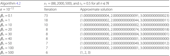
Algorithm 4.2

⎧ ⎪ ⎪ ⎪ ⎪ ⎪ ⎨ ⎪ ⎪ ⎪ ⎪ ⎪ ⎩

x1∈H is given,

zn:=arg minu∈H{g(u) +₂1βnu–xn

2_–_∇_h₍_x

n),u–xn}, yn:=arg minv∈H{g(v) +₂_β1_nv–zn2–∇h(zn),v–zn}, xn+1:= (1 –rn)zn+rnyn, n∈N.

Theorem 4.2 Let{xn}n∈N be generated by Algorithm4.2.Then {xn}n∈N converges to an elementx¯∈ΩDCP.

Example 4.1 Let g,h : R3 _→ _R _{be deﬁned by} _g₍_x

1,x2,x3) := 2x12 + 2x22 + 2x23 and

h(x1,x2,x3) := 4x1+ 8x2 + 12x3 for all (x1,x2,x3)∈R3. Then ΩDCP:={x∈H :∇h(x)∈

∂g(x)}={(1, 2, 3)}.

Example 4.2 Let g1,h1 : R3 → R be deﬁned by g1(x1,x2,x3) := 2x21 + 2x22 + 2x23 and

h1(x1,x2,x3) := 4x1+ 8x2+ 12x3 for all (x1,x2,x3)∈R3. Letg2,h2:R2 →Rbe deﬁned

by g2(y1,y2) :=y12+y22 andh2(y1,y2) := 28y1+ 64y2 for all (y1,y2)∈R2. LetA:R3→R2

be deﬁned byA(x1,x2,x3) = (x1+ 2x2+ 3x3, 4x1+ 5x2+ 6x3) for all (x1,x2,x3)∈R3. Here,

A ≈0.10517 andΩSDCP={(1, 2, 3)}.

From Table1, we see that Algorithm4.2reaches the required errors only need six it-erations ifβn= 500 for alln∈N, but Algorithm4.2reaches the required errors need 73

iterations ifβn= 0.1 for alln∈N.

From Table2, we see that Algorithm4.2reaches the required errors only need seven iterations ifβn= 100 for alln∈N, but Algorithm4.2reaches the required errors need 72

From Table3, we see that Algorithm3.1reaches the required errors only need seven iterations ifβn= 700 for alln∈N, but Algorithm3.1reaches the required errors need 99

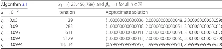
From Table3and Table4, we see that Algorithm3.1reaches the required errors need 283 iterations ifβn= 1 andrn= 0.05 for alln∈N, but Algorithm3.1reaches the required

errors need 39 iterations ifβn= 1 andrn= 0.09 for alln∈N. On the other hand, for other

settings ofβn, we know the numerical results in Table3and Table4show that there are

[image:14.595.117.479.611.732.2]

no signiﬁcant diﬀerences in the setting of{rn}n∈N.

Table 1 Numerical results for Example4.1.

Algorithm4.2 x1= (88, 2000, 500), andrn= 0.5 for alln∈N

ε= 10–12 _Iteration _{Approximate solution}

βn= 0.1 73 (1.00000000000004, 2.00000000000091, 3.00000000000023)

βn= 1 18 (1.00000000000002, 2.00000000000044, 3.00000000000011)

βn= 10 10 (1.00000000000000, 2.00000000000002, 3.00000000000000)

βn= 20 8 (1.00000000000003, 2.00000000000074, 3.00000000000018)

βn= 30 8 (1.00000000000000, 2.00000000000004, 3.00000000000001)

βn= 40 8 (1.00000000000000, 2.00000000000001, 3.00000000000000)

βn= 50 7 (1.00000000000002, 2.00000000000049, 3.00000000000012)

βn= 100 7 (1.00000000000000, 2.00000000000001, 3.00000000000030)

(15)

[image:15.595.117.477.96.207.2]

βn= 0.1 72 (1.00000000000009, 2.00000000000034, 3.00000000000059)

βn= 1 18 (1.00000000000003, 2.00000000000010, 3.00000000000017)

βn= 10 9 (1.00000000000007, 2.00000000000027, 3.00000000000047)

βn= 20 8 (1.00000000000005, 2.00000000000017, 3.00000000000029)

βn= 30 8 (1.00000000000000, 2.00000000000001, 3.00000000000002)

βn= 40 7 (1.00000000000011, 2.00000000000042, 3.00000000000073)

βn= 50 7 (1.00000000000003, 2.00000000000011, 3.00000000000019)

[image:15.595.117.479.254.374.2]

βn= 100 7 (1, 2, 3)

βn= 0.1 99 (0.99999999999927, 1.99999999999990, 3.00000000000052)

βn= 1 39 (1.00000000000036, 2.00000000000048, 3.00000000000059)

βn= 10 15 (1.00000000000018, 2.00000000000024, 3.00000000000030)

βn= 20 12 (0.99999999999973, 1.99999999999964, 2.99999999999955)

βn= 30 11 (1.00000000000013, 2.00000000000017, 3.00000000000021)

βn= 40 10 (0.99999999999963, 1.99999999999952, 2.99999999999940)

βn= 50 10 (0.99999999999995, 1.99999999999993, 2.99999999999992)

βn= 100 9 (1.00000000000001, 2.00000000000002, 3.00000000000002)

βn= 700 7 (1, 2, 3)

βn= 0.1 98 (0.99999999999931, 1.99999999999990, 3.00000000000050)

βn= 1 283 (1.00000000000038, 2.00000000000051, 3.00000000000063)

βn= 10 21 (1.00000000000008, 2.00000000000010, 3.00000000000013)

βn= 20 15 (1.00000000000042, 2.00000000000056, 3.00000000000069)

βn= 30 14 (0.99999999999997, 1.99999999999996, 2.99999999999995)

βn= 40 12 (0.99999999999959, 1.99999999999946, 2.99999999999933)

βn= 50 12 (0.99999999999996, 1.99999999999995, 2.99999999999994)

βn= 100 10 (0.99999999999994, 1.99999999999992, 2.99999999999990)

βn= 1300 7 (1, 2, 3)

Algorithm3.1 x1= (123, 456, 789), andβn= 1 for alln∈N

rn= 0.05 39 (1.00000000000036, 2.00000000000048, 3.00000000000059)

rn= 0.09 283 (1.00000000000038, 2.00000000000051, 3.00000000000063)

rn= 0.095 611 (1.00000000000041, 2.00000000000054, 3.00000000000067)

rn= 0.099 5129 (1.00000000000043, 2.00000000000056, 3.00000000000070)

rn= 0.0994 18,434 (0.99999999999957, 1.99999999999943, 2.99999999999930)

However, in Table5, ifβn= 1 for alln∈N, then we know the numerical results have big

[image:15.595.117.479.421.541.2] [image:15.595.116.477.589.670.2]

(16)

Acknowledgements

The authors would like to thank referee(s) for many useful comments and suggestions for the improvement of the article. Prof. Chi-Ming Chen was supported by Grant No. MOST 107-2115-M-007-008 of the Ministry of Science and Technology of the Republic of China.

Funding Not applicable.

Competing interests

The authors declare that they have no competing interests.

Authors’ contributions

The authors contributed equally and signiﬁcantly in writing this paper. The authors read and approved the ﬁnal manuscript.

Author details

1_{Department of Applied Mathematics, National Chiayi University, Chiayi, Taiwan.}2_{Institute of Computational and}

Modeling Science, National Tsing Hua University, Hsinchu, Taiwan.

Publisher’s Note

Springer Nature remains neutral with regard to jurisdictional claims in published maps and institutional aﬃliations.

Received: 4 October 2018 Accepted: 29 April 2019 References

1. Bauschke, H.H., Combettes, P.L.: Convex Analysis and Monotone Operator Theory in Hilbert Spaces. Springer, Berlin (2011)

2. Butnariu, D., Iusem, A.N.: Totally Convex Functions for Fixed Points Computation and Inﬁnite Dimensional Optimization. Kluwer Academic, Norwell (2000)

3. Byrne, C., Censor, Y., Gibali, A., Reich, S.: Weak and strong convergence of algorithms for the split common null point problem. J. Nonlinear Convex Anal.13, 759–775 (2011)

4. Chuang, C.S.: Strong convergence theorems for the split variational inclusion problem in Hilbert spaces. Fixed Point Theory Appl.2013, 350 (2013)

5. Combettes, P.L., Wajs, V.R.: Signal recovery by proximal forward-backward splitting. Multiscale Model. Simul.4, 1168–1200 (2005)

6. Fujikara, Y., Kuroiwa, D.: Lagrange duality in canonical DC programming. J. Math. Anal. Appl.408, 476–483 (2013) 7. Harada, R., Kuroiwa, D.: Lagrange-type in DC programming. J. Math. Anal. Appl.418, 415–424 (2014)

8. Hiriart-Urruty, J.B., Tuy, H.: Essays on Nonconvex Optimization. Mathematical Programming, vol. 41. North-Holland, Amsterdam (1988)

9. Levy, A.J.: A fast quadratic programming algorithm for positive signal restoration. IEEE Trans. Acoust. Speech Signal Process.31, 1337–1341 (1983)

10. Marino, G., Xu, H.K.: Convergence of generalized proximal point algorithm. Commun. Pure Appl. Anal.3, 791–808 (2004)

11. Martinet, B.: Régularisation d’inéquations variationnelles par approximations successives. Rev. Fr. Inform. Rech. Opér. 4(Ser R–3), 154–158 (1970)

12. Moudaﬁ, A.: Split monotone variational inclusions. J. Optim. Theory Appl.150, 275–283 (2011)

13. Pham, D.T., An, L.T.H., Akoa, F.: The DC (diﬀerence of convex functions) programming and DCA revisited with DC models of real world nonconvex optimization problems. Ann. Oper. Res.133, 23–46 (2005)

14. Saeki, Y., Kuroiwa, D.: Optimality conditions for DC programming problems with reverse convex constraints. Nonlinear Anal.80, 18–27 (2013)

15. Souza, J.C.O., Oliveira, R.P., Soubeyran, A.: Global convergence of a proximal linearized algorithm for diﬀerence of convex functions. Optim. Lett.10, 1529–1539 (2016)

16. Sun, W., Sampaio, R.J.B., Candido, M.A.B.: Proximal point algorithm for minimization of DC functions. J. Comput. Math. 21, 451–462 (2003)