R E S E A R C H
Open Access
A globally convergent QP-free algorithm
for nonlinear semidefinite programming
Jian-Ling Li
1, Zhen-Ping Yang
1and Jin-Bao Jian
2**Correspondence:
[email protected] 2School of Mathematics and
Statistics, Guangxi Colleges and Universities Key Laboratory of Complex System Optimization and Big Data Processing, Yulin Normal University, Jiaoyu Road, Yulin, Guangxi 537000, China Full list of author information is available at the end of the article
Abstract
In this paper, we present a QP-free algorithm for nonlinear semidefinite programming. At each iteration, the search direction is yielded by solving two systems of linear equations with the same coefficient matrix;l1penalty function is
used as merit function for line search, the step size is determined by Armijo type inexact line search. The global convergence of the proposed algorithm is shown under suitable conditions. Preliminary numerical results are reported.
MSC: Primary 90C30; secondary 90C22
Keywords: nonlinear semidefinite programmming; KKT conditions; QP-free algorithm; global convergence
1 Introduction
Consider the following nonlinear semidefinite programming (NLSDP for short):
minf(x)
s.t.A(x);
hj(x) = , j∈E={, , . . . ,l},
(.)
wheref :Rn→R,h
j(j∈E) :Rn→Rl andA:Rn→Smare continuously differentiable functions, not necessarily convex.Sm is a space whose elements are real symmetric ma-trices of sizem×m.denotes the negative semidefinite order, that is,ABif and only ifA–Bis a negative semidefinite matrix.
NLSDP (.) has a broad range of applications such as eigenvalue problems, control problems, optimal structural design, truss design problems (see [–]). So it is desired to develop numerical methods for solving NLSDP (.).
In recent years, NLSDPs have been attracting a great deal of research attention [, –]. As is well known, NLSDP (.) is an extension of nonlinear programming, some efficient numerical methods for the latter are generalized to solve NLSDP. For example, Correa and Ramirez [] proposed an algorithm which used the sequential linear SDP method. Fares et al.[] applied the sequential linear SDP method to robust control problems. Freund et al.[] also studied a sequential SDP method. Kanzowet al.[] presented a successive linearization method with a trust region-type globalization strategy.
In addition, Kovara and Stingl [] developed a computer code PENNON for solving NLSDP (.), where the augmented Lagrangian function method was used. Sunet al.[] and Luoet al.[, ] proposed an augmented Lagrangian method for NLSDP (.), re-spectively. Sunet al. [] analyzed the rate of local convergence of the augmented La-grangian method for NLSDPs. Yamashitaet al.recently proposed a primal-dual interior point method for NLSDP (.) (see []). The algorithm is globally convergent and lo-cally superlinearly convergent under suitable conditions. Very recently Aroztegui [] pro-posed a feasible direction interior point algorithm for NLSDP (.) with only semidefinite matrix constraint.
As we know, QP-free (also called SSLE) method is a kind of efficient methods for stan-dard nonlinear programs (see []-[]). In this paper, motivated from QP-free method for standard nonlinear programs, based on techniques of perturbation and penalty function, we propose a globally convergent QP-free algorithm for NLSDP (.). The construction of systems of linear equations (SLE for short) is a key point. Based on KKT conditions of NLSDP (.) and techniques of perturbation, we construct two SLEs skillfully. At each iteration, the search direction is yielded by solving two SLEs with the same coefficient ma-trix; An exact penalty function is used as the merit function for line search and the step size is determined by suitable inexact line search. The global convergence of the proposed algorithm is shown under some mild conditions.
The paper is organized as follows. In Section we restate some definitions and results on NLSDP and matrix analysis. In Section the algorithm is presented and its feasibility is discussed. The global convergence is analyzed in Section . Some preliminary numer-ical results are reported in Section and some concluding remarks are given in the final section.
2 Preliminaries
For the sake of convenience, some results on matrix analysis and NLSDP are restated in this section, which will be employed in the following analysis of the proposed algorithm. More introduction for theory of matrices should be seen in [] and []. Denote byRm×n the space ofm×nreal matrices, denote byS+m andS++m the sets ofm-order symmetric positive semidefinite and positive definite matrices, respectively. The setsSm
– andS––m are defined similarly.
Definition . For anyA= (aij),B= (bij)∈Rm×n, the inner product ofAandBis defined by
A,B=TrBTA= m
i= n
j=
aijbij, (.)
whereTr(P) means the trace of the matrixP.
Definition .([]) For anyM∈Rm×m, let
sym(M) =
M+MT, skw(M) =
M–MT, (.)
Given a matrixA∈Sm, letm=
m(m+ ), define a mapsvec:Sm→Rm:
svec(A) = (a,
√
a, . . . ,
√
am,a,
√
a, . . . ,
√
am, . . . ,amm)T,
and the mapsmat:Rm→Smis defined to be the inverse ofsvec. Then the inner product of matrices is indicated by
A,B=svec(A)Tsvec(B), forA,B∈Sm. (.)
Definition .([]) For anyA,B∈Rm×m, the symmetric Kronecker product, denoted by A⊗sB, is a mapping on a vectoru=svec(U) whereUis anm×msymmetric matrix and is defined as
(A⊗sB)u= svec
BUAT+AUBT. (.)
For any matrixU∈Sm, it is verified that the following equality is true:
(A⊗sB)svec(U) =svec
sym(BUA). (.)
Note that the linear operatorA⊗sBis defined implicitly in (.). In Appendix of [] a matrix representation ofA⊗sBis given as follows:
A⊗sB=
Q(A⊗B+B⊗A)Q
T, (.)
whereA⊗B= [aijB] (i,j= , , . . . ,m) is the Kronecker product ofAandB,Qis an orthog-onalm×mmatrix (i.e. QQT=I
m), with the following property:
Qvec(U) =svec(U), QTsvec(U) =vec(U), ∀U∈Sm, (.)
wherevec(U) = (u,u, . . . ,um,u,u, . . . ,um, . . . ,umm)T.
Remark . One choice for the matrixQis given in the appendix of [].
Lemma .([]) For any A,B∈Sm,the following results are true: () A⊗sB=B⊗sA;
() (A⊗sB)T=AT⊗sBT;
() (A⊗sB)(C⊗sD) =(AC⊗sBD+AD⊗sBC);
() IfAandBare symmetric positive definite,thenA⊗sBis positive definite.
Lemma .([]) If A,B∈Sm,Aand AB+BA≺,then B≺.
Lemma . If A∈Sm
++,B∈S––m,then all eigenvalues of AB are less than zero.
The proof is elementary and omitted here.
Lemma . Suppose A∈Sm
++,B∈S––m,and they commute,then(A⊗sIm)–(B⊗sIm)∈S––m.
Proof SinceA∈Sm
++,B∈S––m, and they commute, there exists an orthogonal matrixP∈ Rm×msuch that
A=PDAP–, B=PDBP–,
where DA is a diagonal and positive definite matrix, andDB is a diagonal and negative definite matrix. It follows from Lemma .() that
A⊗sIm=T DAT–, B⊗sIm=T DBT–,
whereT =P⊗sP,DA=DA⊗sImandDB=DB⊗sIm. We know from Lemma .(), () thatT is orthogonal, from Lemma .() thatDAis a diagonal and positive definite matrix, andDBis a diagonal and negative definite matrix. Hence,
(A⊗sIm)–(B⊗sIm) =T DADBT–∈S––m.
In the rest of this section we state the first order optimality conditions for NLSDP (.). For the sake of convenience, we first introduce some notations. Given a matrix valued functionA(·), we use the notation
DA(x) =
∂A(x) ∂x
, . . . ,∂A(x)
∂xn
T
for its differential operator evaluated atx, where ∂A∂x(x)
i denotes the partial derivative of
A(x) with respect toxi with components ∂apq(x)
xi (p,q= , . . . ,m). Then the derivative of
A(·) in the directiond= (d, . . . ,dn)T∈Rnatxdenoted byDA(x)dis defined by
DA(x)d= n
i= di
∂A(x) ∂xi
. (.)
If we denote
∇A(x) :=
svec
∂A(x) ∂x
, . . . ,svec
∂A(x) ∂xn
m×n
, (.)
then by (.), the following equality is true:
svecDA(x)d=∇A(x)d. (.)
The Lagrangian function of NLSDP (.)L:Rn×Sm×Rl→Ris defined by
L(x,,μ) =f(x) +A(x),+h(x)Tμ, (.) whereh(x) = (h(x),h(x), . . . ,hl(x))T. In view of (.), the above equality can be rewritten as follows:
whereλ:=svec(). The gradient ofL(x,λ,μ) with respect toxis given as follows:
∇xL(x,λ,μ) =∇f(x) +∇A(x)Tλ+∇h(x)μ, (.)
where∇h(x) = (∇h(x),∇h(x), . . . ,∇hl(x)).
We are now in a position to restate the definition of the first order optimality conditions for NLSDP (.).
Definition .([]) Forx∈Rn, if there exist a matrix∈Smand a vectorμ(∈Rl) such that
∇xL(x,,μ) = , (.a)
A(x) = , , (.b)
h(x) = , A(x), (.c)
thenxis called a KKT point of NLSDP (.).
Remark . According to the Von Neumann-Theobald inequality, the complementarity conditionA(x) = has the following two useful equivalent forms:
TrA(x)= ,
λj()λj
A(x)= , ∀j∈ {, , . . . ,m}.
3 The algorithm
In this section, we present our algorithm and show it is well defined. For the sake of sim-plicity, we introduce some notations:
= x∈Rn:A(x),h(x) = ,
F= x∈Rn:A(x), F= x∈Rn:A(x)≺
,
that is,is the feasible set of NLSDP (.).
In general,A(x) is not guaranteed to be symmetric, so we considersym(A(x)) =
instead ofA(x) = . Then the three equalities of KKT condition (.a)-(.c) can be
rewritten in the following form:
∇f(x) +∇A(x)Tλ+∇h(x)μ= ,
svecsymA(x)= , h(x) = .
(.)
In order to solve (.) at each Newton iteration, we define a vector-value functionϕ: Rn+m+l→Rn+m+las follows:
ϕ(x,λ,μ) =
⎛ ⎜ ⎝
ϕLg(x,λ,μ)
ϕC(x,λ,μ)
ϕh(x,λ,μ)
⎞ ⎟ ⎠=
⎛ ⎜ ⎝
∇f(x) +∇A(x)Tλ+∇h(x)μ svec(sym(A(x)))
h(x)
It follows from (.) and Lemma . that
ϕC(x,λ,μ) =svec
symIA(x)=I⊗sA(x)
svec() = (⊗sI)svec
A(x),
thus, the Jacobian ofϕis
∇ϕ(x,λ,μ) =
⎛ ⎜ ⎝
∇
xxL(x,λ,μ) ∇A(x)T ∇h(x) (⊗sI)∇A(x) I⊗sA(x)
∇h(x)T
⎞ ⎟ ⎠.
Instead of the Hessian∇
xxL(x,λ,μ), we employ a positive definite matrix denoted byH which can be a quasi-Newton approximation or the identity matrix. A Newton-like itera-tion to solve (.) is given by the linear systems as follows:
⎛ ⎜ ⎝
H ∇A(x)T ∇h(x) (⊗sI)∇A(x) I⊗sA(x)
∇h(x)T
⎞ ⎟ ⎠
⎛ ⎜ ⎝
x–x
λ–λ
μ–μ
⎞ ⎟ ⎠
= –
⎛ ⎜ ⎝
∇f(x) +∇A(x)Tλ+∇h(x)μ
svec(sym(A(x)))
h(x)
⎞ ⎟
⎠, (.)
where (x,,μ)∈F×S++m ×Rlis the current point, (x,,μ)∈F×S++m ×Rlis the new estimates given by the Newton-like iteration, λ:=svec() andλ:=svec(). Let d=x–x, we obtain from (.)
Hd+∇A(x)Tλ+∇h(x)μ= –∇f(x), (.a)
(⊗sI)∇A(x)d+
I⊗sA(x)
λ= , (.b)
∇h(x)Td= –h(x). (.c)
Ifd= , then we have
∇f(x) +∇A(x)Tλ+∇h(x)μ= ,
I⊗sA(x)
λ= , h(x) = .
SinceA(x)≺,I⊗sA(x) is nonsingular and we have:=smat(λ) = , which implies thatA(x) = . Therefore,xis a KKT point. Ifd= , thendis not guaranteed to be a feasible direction. To obtain a better search direction, we modify (.b) by introducing an appropriate right hand side, so we obtain another linear equations as follows:
Hd+∇A(x)Tλ+∇h(x)μ= –∇f(x),
(⊗sI)∇A(x)d+
I⊗sA(x)
λ= –λd,
∇h(x)Td= –h(x).
(.)
A For anyx∈F,the matrix
B(x) =
∇A(x)T ∇h(x) A(x)⊗sIm
is full of column rank.
The following lemma gives a sufficient condition of the assumption A.
Lemma . For any x∈F,ifA(x)≺and{∇h(x), . . . ,∇hl(x)}is linearly independent,
then B(x)is full of column rank,i.e.,the assumptionAholds.
Lemma . Let H be a positive definite matrix.If the assumptionAholds,then the coef-ficient matrix of the SLEs(.a)-(.c)and(.)
W(x,H,)def=
⎛ ⎜ ⎝
H ∇A(x)T ∇h(x) (⊗sIm)∇A(x) A(x)⊗sI
∇h(x)T
⎞ ⎟
⎠ (.)
is nonsingular,hence,SLEs(.a)-(.c)and(.)have a unique solution,respectively.
The proof is elementary and it is omitted here.
In our algorithm the following exact penalty function is used as a merit function for line search:
P(x;σ) =f(x) +σ
j∈E
hj(x), (.)
whereσ > is a penalty parameter. Further, we define a functionP(•;d;σ) :Rn×Rn× [, +∞)→Rassociated withP(x;σ) by
P(x;d;σ) =f(x) +∇f(x)Td+σ
j∈E
hj(x) +∇hj(x)Td. (.)
Now the algorithm is described in detail.
Algorithm A
Parameters.α∈(,),β,ξ∈(, ),λI> ,σ–> ,ρ,ρ> . Initialization. Select an initial iteration pointx∈F
, H∈S++n , (∈S++m) satisfying
λIImsuch thatandA(x) commute. Letλ=svec(),k:= .
Step . Let(dk,λk,μk)be the solution of the SLE (.a)-(.c) in(d,λ,μ),i.e.,
⎧ ⎪ ⎪ ⎨ ⎪ ⎪ ⎩
Hkd+∇A(xk)Tλ+
j∈Eμj∇hj(xk) = –∇f(xk), (k⊗sIm)∇A(xk)d+ (A(xk)⊗sIm)λ= ,
∇hj(xk)Td= –hj(xk), j∈E.
(.)
Step . Let(dk,λk,μk)be the solution of the SLE (.) in(d,λ,μ),i.e.,
⎧ ⎪ ⎪ ⎨ ⎪ ⎪ ⎩
Hkd+∇A(xk)Tλ+
j∈Eμj∇hj(xk) = –∇f(xk), (k⊗sIm)∇A(xk)d+ (A(xk)⊗sIm)λ= –λkdk,
∇hj(xk) T
d= –hj(xk), j∈E.
(.)
Step . Compute the search directiondkand the approximate multiplier vector(λk,μk):
dk= ( –δk)dk+δkdk, (.)
λk= ( –δk)λk+δkλk, (.)
μk= ( –δk)μk+δkμk, (.)
where
δk=
⎧ ⎪ ⎪ ⎨ ⎪ ⎪ ⎩
–ξ, if∇f(xk)Tdk≤;
, if∇f(xk)Tdk> and∇f(xk)Tdk≤ ∇f(xk)Tdk;
min{ξ,|( –ξ)∇f(∇xk)Tdk+(μk)Th(xk)
f(xk)T(dk–dk) |}, otherwise.
(.)
Step . (Update the penalty parameter) Setσk= ( –ξ)maxj∈E|μkj|+ρ. The updating
rule ofσkis as follows:
σk=
⎧ ⎨ ⎩
max{σk,σk–+ρ}, ifσk>σk–,
σk–, otherwise.
(.)
Step . (Line search) Set the step sizetkto be the first number of the sequence{,β,β, . . .} satisfying the following two inequalities:
Pxk+tdk;σk
≤Pxk;σk
+tαPxk;dk;σk
–Pxk; ;σk
, (.)
Axk+tdk≺. (.)
Step . Setxk+=xk+t
kdk. Using the following methods to generatek+commuting with A(xk+):
Step .. If the search directiondkdoes not descend or is not feasible, set k+=Im and go to Step .
Step .. Compute the least eigenvalueλmin(k)of the matrix¯k. Ifλmin(k)≥λI, then letk+=k; otherwise, letk+=k+ (λI–λmin(k))Im.
Step . Set λk+=svec(k+), and updateHk by some method toHk+ such thatHk+ is
symmetric positive definite. Letk:=k+ , return to Step .
Lemma . Suppose that the assumptionAholds.If dk= ,then xkis a KKT point of NLSDP(.).
Lemma . Suppose that the assumptionAholds.Then the search direction dkof Algo-rithmAsatisfies the following inequality:
∇fxkTdk≤–ξdkTHkdk+ ( –ξ)
j∈E
μkjhj
xk. (.)
Proof First we show that the inequality
∇fxkTdk≤–dkTHkdk+
j∈E
μkjhj
xk (.)
holds. Premultiplying the first equation of (.) by (dk)T, we obtain
dkTHkdk+
j∈E
μkjdkT∇hj
xk+dkT∇AxkTλk= –dkT∇fxk. (.)
According to the second equation of (.), we get
dkT∇AxkTλk= –λkT(k⊗sIm)–
Axk⊗sIm
T
λk.
Substituting the above equality and the third equality of (.) into (.), we have
dkT∇fxk = –dkTHkdk+
λkT(k⊗sIm)–
Axk⊗sIm
T
λk+ j∈E
μkjhj
xk.
In view of Lemma ., the matrix (k⊗sIm)–(A(xk)⊗sIm) is negative semidefinite, so it follows from the above equality that
dkT∇fxk≤–dkTHkdk+
j∈E
μkjhj
xk,
i.e., the inequality (.) holds.
Next, we will prove the inequality (.) is true. The rest of the proof is divided into three cases.
CaseA.∇f(xk)Tdk≤. From (.) we haveδk= –ξ. It follows from (.), (.), (.) andξ∈(, ) that
∇fxkTdk≤–ξdkTHkdk+ξ
j∈E
μkjhj
xk
≤–ξdkTHkdk+ ( –ξ)
j∈E
μkjhj
xk, (.)
Case B.∇f(xk)Tdk> and ∇f(xk)Tdk≤ ∇f(xk)Tdk. From (.), one hasδ k = . It follows from (.), (.) andξ∈(, ) that
∇fxkTdk =∇fxkTdk≤ ∇fxkTdk
≤–dkTHkdk+
j∈E
μkjhj
xk,
which implies (.) holds.
CaseC.∇f(xk)Tdk> and∇f(xk)Tdk>∇f(xk)Tdk. It follows from (.) andξ∈(, ) that
δk=
( –ξ)∇f(x
k)Tdk+ (μk)Th(xk)
∇f(xk)T(dk–dk)
≤ |(ξ– )∇∇f(xk)Tdk|+|(μk)Th(xk)|
f(xk)T(dk–dk) . (.)
If∇f(xk)Tdk≤, then we obtain from the above inequality
( –δk)∇f
xkTdk+δk∇f
xkTdk≤ξ∇fxkTdk+μkThxk, which together with (.) and (.) gives
∇fxkTdk≤–ξdkTHkdk+ ( +ξ)
j∈E
μkjhj
xk
≤–ξdkTHkdk+ ( –ξ)
j∈E
μkjhj
xk. (.)
If∇f(xk)Tdk> , then the inequality (.) gives rise to
δk∇f
xkTdk–δk∇f
xkTdk≤( –ξ)∇fxkTdk+μkThxk, which together with (.) and (.) shows
∇fxkTdk≤–( –ξ)dkTHkdk+ ( –ξ)
j∈E
μkjhj
xk
≤–ξdkTHkdk+ ( –ξ)
j∈E
μkjhj
xk. (.)
The inequalities (.) and (.) indicate that the inequality (.) is true.
Lemma . Suppose that the assumptionAholds.If xk(∈F)is not a KKT point of NLSDP (.),then
Pxk;dk;σk
–Pxk; ;σk
< . (.)
Proof From (.) and (.) we know that (dk,λk,μk) is the solution of the following SLE:
Hkd+∇A
xkTλ+ j∈E
μj∇hj
(k⊗sIm)∇A
xkd+Axk⊗sIm
λ= –δkλkdk, (.b)
∇hj
xkTd= –hj
xk, j∈E. (.c) From the definition (.) of the functionP(xk;dk;σk) and (.c), we have
Pxk;dk;σk
–Pxk; ;σk
=∇fxkTdk–σk
j∈E
hj
xk
≤–ξdkTHkdk+ ( –ξ)
j∈E
μkjhj
xk–σk
j∈E
hj
xk
≤–ξdkTHkdk+
( –ξ)max j∈E
μkj–σk j∈E
hj
xk, (.)
the first inequality above is due to (.).
Sincexkis not a KKT point of NLSDP (.), it implies from Step of Algorithm A that dk= , so (dk)TH
kdk> . On the other hand, it follows from the updating rule ofσkthat
σk> ( –ξ)maxj∈E|μkj|, therefore, (.) gives rise to
Pxk;dk;σk
–Pxk; ;σk
< ,
that is, the inequality (.) holds.
Lemma . Suppose that the assumptionAholds.If AlgorithmAdoes not stop at the current iterate xk,then(.)and(.)are satisfied for t> small enough,so AlgorithmA is well defined.
Proof It follows from the Taylor expansion and (.) that
Pxk+tdk;σk
–Pxk;σk
=t∇fxkTdk+σk
j∈E
hj
xk+t∇hj
xkTdk–hj
xk+o(t)
=Pxk;tdk;σk
–Pxk; ;σk
+o(t). (.)
The second equality above is due to (.). From the convexity ofP(xk;d;σ
k) ford, we obtain
Pxk;tdk;σk
–Pxk; ;σk
≤tPxk;dk;σk
–Pxk; ;σk
, (.)
which together with (.) and Lemma . gives fortsmall enough
Pxk+tdk;σk
–Pxk;σk
≤tαPxk;dk;σk
–Pxk; ;σk
,
whereα∈(, ). Hence, (.) holds for sufficiently smallt> .
In what follows, we prove (.) holds for sufficiently small t> . SinceA(x) is twice continuously differentiable function, it follows from Taylor expansion that
Note that the largest eigenvalue functionλmax(A) =maxv=vTAv, we deduce from (.) andA(xk)≺ that
λmax
Axk+tdk=max v= v
TAxkv+vTO(t)v<
for <t< small enough, which implies (.) holds for <t< small enough.
By summarizing the above discussions, we conclude that Algorithm A is well defined.
4 Global convergence
If Algorithm A terminates at xk after a finite number of iterations, we know from Lemma . thatxk is a KKT point of NLSDP (.). In this section, without loss of gen-erality, we assume that the sequence{xk}generated by Algorithm A is infinite. We will prove any accumulation point of{xk}is a stationary point or a KKT point of NLSDP (.), i.e., Algorithm A is globally convergent. We first generalize the definition of stationary point for nonlinear programming defined in [] to nonlinear semidefinite programming.
Definition . Letx∈Rn, if there exist a matrix(∈Sm) and a vectorμ(∈Rl) such that
∇xL(x,,μ) = , (.)
A(x) = , A(x), h(x) = , (.)
thenxis called a stationary point of NLSDP (.).
In order to analyze the global convergence, some additional assumptions are required: A The sequence{xk}yielded by AlgorithmAlies in a nonempty closed and bounded
setX.
A The functionsf(x),h(x)andA(x)are twice continuously differentiable on an open set containingX.
A There exists a positive constantλssuch thatλs>λI andλIImkλsImfor allk. A The matrixHkis uniformly positive definite, i.e., there exist two positive constantsa
andbsuch thatay≤yTH
ky≤byfor ally∈Rn.
Letx∗ be an accumulation point of{xk}, then there exists a subsetK⊆ {, , . . .}such thatlimk∈Kxk=x∗. Without loss of generality, we suppose
Hk
K
−→H∗, ∇hxk−→ ∇K hx∗,
k
K
−→∗, Wxk,Hk,k
K
−→Wx∗,H∗,∗,
whereW(xk,H
k,k) is defined by (.) and
Wx∗,H∗,∗def=
⎛ ⎜ ⎝
H∗ ∇A(x∗)T ∇h(x∗) (∗⊗sIm)∇A(x∗) A(x∗)⊗sIm
∇h(x∗)T
⎞ ⎟ ⎠.
Lemma . Suppose the assumptionsA-Ahold.Then there exists a constant M> such that|f(yk)| ≤M,∇f(yk) ≤M,∇f(yk) ≤M,h(yk) ≤M,∇h(yk) ≤M,A(yk)
F≤ M,DA(yk)
F≤M andDA(yk)F≤M,for any yk∈N(xk),whereN(xk)is a neighbor-hood of xk.
Lemma . Suppose the assumptionsA-Ahold.Then
() there exists a constantc> such thatW(xk,Hk,k)– ≤cfor anyk∈K;
() there exists a constantM> such thatλk ≤M,λk ≤M,μk ≤M,
μk ≤M,dk ≤Manddk ≤Mfor anyk∈K.
The following result is an important property of the penalty parameterσk, which is ob-tained by the updating rule (.).
Lemma . Suppose the assumptionsA-Ahold.Then the penalty parameterσkis up-dated only in a finite number of steps.
Based on Lemma ., in the rest of the paper, we assume, without loss of generality, that
σk≡ ˜σfor allk, where
˜
σ>sup k
( –ξ)max j∈E
μkj.
By using of Lemma ., we obtain the following result.
Lemma . Suppose the assumptionsA-Ahold.Then there exists a constant c> such that
dk–dk≤cdk. (.)
For the sake of simplicity, in the rest of this section, let (d∗,μ∗,λ∗) be the solution of the following SLE in (d,μ,λ):
⎧ ⎪ ⎪ ⎨ ⎪ ⎪ ⎩
H∗d+∇A(x∗)Tλ+j∈Eμj∇hj(x∗) = –∇f(x∗), (∗⊗sIm)∇A(x∗)d+ (A(x∗)⊗sIm)λ= ,
∇hj(x∗)Td= –hj(x∗), j∈E.
(.)
Let (d∗,μ∗,λ∗) be the solution of the following SLE in (d,μ,λ):
⎧ ⎪ ⎪ ⎨ ⎪ ⎪ ⎩
H∗d+∇A(x∗)Tλ+j∈Eμj∇hj(x∗) = –∇f(x∗), (∗⊗sIm)∇A(x∗)d+ (A(x∗)⊗sIm)λ= –λ∗d∗,
∇hj(x∗)Td= –hj(x∗), j∈E.
(.)
From the above equalities and Lemma ., we obtain the following conclusion.
Lemma . Suppose the assumptionsA-Ahold,andδk
K
(ii) dk−→K d∗,μk−→K μ∗,λk−→K λ∗,
(iii) d∗= if and only ifd∗= whered∗= ( –δ∗)d∗+δ∗d∗.
Remark . By (.), we know that{δk}is bounded, so in the rest of the paper, we assume,
without loss of generality, thatδk
K −→δ∗.
Lemma . Suppose the assumptionsA-Ahold.Let x∗be an accumulation point of the sequence{xk}and xk−→K x∗.If dk−→K ,then x∗is a KKT point or a stationary point of NLSDP(.),andλk−→K svec(∗),μk−→K μ∗,where(∗,μ∗)is the Lagrangian multiplier corresponding to x∗.
Proof It is clear from Lemma . that{λk}and{μk}are bounded. Assume thatλˆ,μˆ are accumulation points of{λk}and{μk}, respectively. Without loss of generality, we assume
thatλk−→ ˆK λandμk−→ ˆK μ.
Obviously, (dk,λk,μk) satisfies the SLE (.a)-(.c). By taking the limit on K in (.a)-(.c), we obtain
∇Ax∗λˆ+ j∈E
ˆ
μj∇hj
x∗= –∇fx∗, (.a)
Ax∗⊗sI
ˆ
λ= , (.b)
hj
x∗= , j∈E. (.c)
Ifx∗∈F,i.e.,A(x∗)≺, then we know from Lemma .() thatA(x∗)⊗sIis nonsingular, so the equation (.b) has a unique solutionλˆ = . Let:=smat(λˆ) = , soA(x∗) = . Together with (.a) and (.c), we conclude thatx∗is a KKT point of NLSDP (.).
Ifx∗∈\F, let:=smat(λˆ). It follows from (.b) thatsym(A(x∗)) = , which means thatA(x∗) is a skw-symmetric matrix. HenceTr(A(x∗)) = . According to Remark ., we obtainA(x∗) = . Combining with (.a) and (.c),x∗is a stationary point of NLSDP (.). (λ∗,μ∗) is the Lagrangian multiplier corresponding tox∗, that is,
∇Ax∗Tλ∗+ j∈E
μ∗j∇hj
x∗= –∇fx∗,
∗Ax∗= ,
where∗=smat(λ∗). It is not difficult to verify that (λ∗,μ∗) is the solution of the following SLE:
∇Ax∗Tλ∗+ j∈E
μ∗j∇hj
x∗= –∇fx∗, (.a)
Ax∗⊗sI
λ∗= . (.b)
From (.a)-(.c), we know that (λˆ,μˆ) is also the solution of (.a)-(.b). It is clear from the assumption A that the solution of (.a)-(.b) is unique, therefore,λˆ =λ∗,μˆ =μ∗.
The proof is completed.
Lemma . Suppose the assumptionsA-Ahold.Let xk−→K x∗.If dk–−→K ,then x∗is a KKT point or a stationary point of NLSDP(.).
Lemma . Suppose the assumptions A-Ahold, xk−→K x∗. IfinfK{dk–}> ,then dk−→K .
Proof By contradiction, we assume that there exist a subsetK⊂Kand a constantd¯> such thatdk ≥ ¯d,∀k(∈K) large enough. From the assumptions A-A, (.) and the updating rule ofk, we assume without loss of generality thatHk
K
−→H∗,δk
K
−→δ∗,k
K
−→
∗. On the other hand, it follows from the updating rule ofkand the assumption A that
∗is positive definite. According to Lemma .(iii), there existsd> such thatdk ≥d for allk∈K.
Firstly, we show that there existst> independent ofksuch that (.) and (.) are satisfied for allt≥t. For anyk∈K, it is clear from the assumptions A and A and Lem-mas .-. and LemLem-mas .-. that
Pxk;dk;σ˜–Pxk; ;σ˜≤–ξad. (.)
Together with (.)-(.), there existstf > independent ofksuch that
Pxk+tdk;σ˜–Pxk;σ˜≤tαPxk;dk;σ˜–Pxk; ;σ˜ (.) for allk∈Kandt∈(,tf], whereα∈(, ). The above inequality shows the inequality (.) holds.
We next prove the inequality (.) holds. It follows from (.) and Lemma .() and Lemma . that
∇fxkTdk+μkThxk
=–dkTHkdk+
λkT(k⊗sIm)–
Axk⊗sIm
T
λk
≥adk.
Combining with Lemmas .-. and (.), there exists a constant <δ˜≤ such that
δk≥ ˜δfork∈K. By the mean-value theorem and Lemmas .-., we obtain
Axk+tdk=Axk+tDAxkdk+tDAx+tϑdkdk,dk
Axk+tDAxkdk+tMIm (.)
for any k∈K, where ϑ∈(, ), M= max{M, M}. LetN(t;xk) =A(xk) +tDA(xk)dk+ tMI
m, the above inequality is rewritten as
Axk+tdkNt;xk, (.)
thus, in order to prove thatA(xk+tdk) is negative definite, it is sufficient to prove that N(t;xk) is negative definite. In view of
it is sufficient to show that there existstA> independent ofksuch that
symkN
t;xk≺, ∀t∈(,tA]. (.) In view of (.), (.) and Lemma .(), we obtain
(k⊗sIm)∇A
xkdk=svecsymkDA
xkdk. (.) Letk=smat(λk),i.e.,λk=svec(k), it is obvious from (.) that
Axk⊗sIm
λk=Axk⊗sIm
sveck=svecsymkAxk. (.) Hence, (.), (.) and (.b) give rise to
symkDA
xkdk+kAxk =smatsvecsymkDA
xkdk+svecsymkAxk =smat–δkλkdk= –δkdkk.
Based on the above equality, we have
symkN
t;xk=symk
Axk+tDAxkdk+tMIm
=symk–tk
Axk+tMk–tδkdkk
≺symk–tk
Axk+tM–tδ˜dk; (.)
note the positive definiteness ofk, hence, if
max vTk–tk
Axkv:v∈Rm,v= ≤, for anyk∈K, (.)
then (.) holds fort≤δM˜d.
SincekandA(xk) are symmetric and commuting, there exists an orthogonal matrix Qksuch that
k=QTkD k
λQk, A
xk=QTkDkAQk, (.) whereDkλandDkAare diagonal matrices. Then (k–tk)A(xk) =QTk(D
k
λ–tQkkQTk)× DkAQk. Let!k=QkkQTk, so in order to prove (.), it is enough to show that there exists a constanttA> such that
vTDkλ–t!k
DkAv≤, ∀v:v= , (.) for anyt∈(,tA) andk∈K. By Lemma . andk=smat(λk), we know{k}is bounded, furthermore,{!k}is also bounded. Let!∗be an accumulation point of{!k}. Without loss of generality, we assume that!k K
−→!∗. LetBk=!k–!∗, obviously,Bk K
−→, thus there existsγ > such that
for anyk∈K. Note that
vTDkλ–t!k
DkAv=vTDkλ–t!∗
DkAv–tvTBkDkAv. (.)
It follows from the assumption A that all eigenvalues ofDkλare betweenλI andλsfor allk. According to Weyl’s theorem (see []), there existst> such that all eigenvalues of (Dkλ–t!∗) are positive for anyt∈(,t]. We also know fromA(xk)≺ and the second equality in (.) thatDAis negative definite. Therefore, for anyvwithv= andt∈ (,t], it follows from Lemma . that (D
k
λ–t!∗)DkAis also negative definite. Combining with (.), for anyvwithv= and anyt∈(,t), we obtain
vTDkλ–t!∗
DkAv–tvTBkDkAv≤, (.)
together with (.) shows that (.) is satisfied, further, (.) and (.) hold.
LettA= min{t,mdM}, thus (.) holds for anyt∈(,tA]. Hence, we see thatA(xk+
tdk)≺ holds fort∈(,tA] and anyk∈K. Let¯t= min{tf,tA}, for anyt∈(,¯t], (.) and (.) are satisfied for allt≥t. Combining with (.) and (.), we obtain for any k∈K
Pxk+;σ˜≤Pxk;σ˜–tαξad. (.)
On the other hand, the sequence {P(xk;σ˜)} decreases monotonically and P(xk;σ˜)−→K P(x∗;σ˜), so{P(xk;σ˜)}∞
k=is convergent. Letlimk→∞P(xk;σ˜) =and taking the limit in the above inequality, we have –tξ αad≥, which is a contradiction. Hence,dk−→K .
Based on Lemmas .-., the following global convergence of Algorithm A is immedi-ate.
Theorem . Suppose the assumptionsA-Ahold.Then AlgorithmAeither terminates in a finite number of iterations at a KKT point of the NLSDP(.),or it generates a sequence
{xk}whose every accumulation point is a KKT point or a stationary point of the NLSDP (.).
5 Numerical experiments
Algorithm A has been implemented in Matlab b and the codes have been run on a . GHz Intel(R) Core(TM)i- machine with a Windows system. We chooseHas n-order identical matrix and at each iteration,Hkis updated by the damped BFGS formula in [] andasm-order identical matrix. In the numerical experiments, we choose the parameters as follows:
α= ., β= ., ξ= ., λI= .,
σ–= ., ρ= , ρ= .
The stop criterion isdk ≤–.
I. The first test problem is Rosen-Suzuki problem [] combined with a negative semidefinite constraint and denoted byCM:
minf(x) =x+x+ x+x– x– x– x+ x
s.t.x+x+x+x+x–x+x–x– = ,
x+ x+x+ x–x–x– = ,
x
+x+x+ x–x–x– = ,
⎛ ⎜ ⎜ ⎜ ⎝
–x–x –x –x –x –x –x–x
⎞ ⎟ ⎟ ⎟ ⎠.
II. We select some test problems from [] only with equality constraints and we add a negative semidefinite matrix constraint.
() We select the problems HS, HS, HS, HS combined with the following× order symmetric matrix which comes from [] and rename them MHS, MHS, MHS and MHS, respectively:
–x –x –x
–x
.
() Choose the problems HS, HS, HS and HS combined with the following ×order symmetric matrix and rename them MHS, MHS, MHS and MHS, respectively:
⎛ ⎜ ⎝
–x
–x –x
–x
–x
⎞ ⎟ ⎠.
() Choose the problems HS, HS, HS, HS, HS, HS, HS and HS, adding the negative semidefinite matrix constraint in the problemCMand renaming them MHS, MHS, MHS, MHS, MHS, MHS, MHS and MHS. III. Nearest correlation matrix problem (NCM for short) (see []):
minf(X) =
X–AF
s.t.XI,
Xii= , i= , , . . . ,m,
Table 1 The numerical results of test problems I and II
Problem n l m x0 Iter. NF NC ffinal Time (s)
CM 4 3 4 (2.5, 2.5, 2.5, –2.5)T 19 72 72 –4.400000e+001 4.097408e–001 PHS6 2 1 2 (–2, –2)T 99 128 128 1.226381e–006 3.541575e–001 PHS7 2 1 2 (1, 5)T 43 169 169 –1.732051e+000 3.551911e–001
PHS8 2 2 2 (1, 4)T 4 4 4 –1 2.195229e–001
PHS9 2 1 2 (–4, 4)T 2 2 2 –4.999996e–001 2.025914e–001
PHS26 3 1 3 (1.5, 1.5, 1.5)T 28 28 28 3.726010e–005 2.514937e–001 PHS27 3 1 3 (–1, 1, 1)T 17 17 17 5.426241e–002 2.354974e–001 PHS28 3 1 3 (1, –1, –1)T 6 6 6 6.756098e–001 1.708627e–001 PHS40 4 3 4 (0.5, 0.5, 0.5, 0.5)T 8 10 10 –2.500001e–001 2.773717e–001 PHS42 4 2 4 (–1, 1, 1, 1)T 17 28 28 1.385766e+001 2.415490e–001 PHS47 5 3 4 (–1, 1, 1, 1, 1)T 31 80 80 2.910505e–001 2.642828e–001 PHS48 5 2 4 (3, 3, 3, 3, –3)T 49 140 140 3.060758e–008 2.962501e–001 PHS50 5 3 4 (–3, 3, 3, 3, 3)T 23 84 84 2.390072e–009 3.139633e–001 PHS51 5 3 4 (–1, 1, 1, 1, 1)T 13 14 14 4.687353e–008 2.302719e–001 PHS61 3 2 3 (2.5, 2.5, 2.5)T 59 59 59 –8.191909e+001 3.401501e–001 PHS77 5 2 4 (1, 1, 1, 1, 1)T 23 25 25 2.415051e–001 2.393263e–001 PHS79 5 3 4 (–1, 1, 1, 1, 1)T 44 50 50 7.877716e–002 3.415668e–001
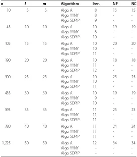
Table 2 The numerical results for NCM problem
n l m Algorithm Iter. NF NC
10 5 5 Algo. A 8 15 15
Algo. YYNY 8 -
-Algo. SDPIP 9 -
-45 10 10 Algo. A 10 19 19
Algo. YYNY 8 -
-Algo. SDPIP 10 -
-105 15 15 Algo. A 10 20 20
Algo. YYNY 10 -
-Algo. SDPIP 11 -
-190 20 20 Algo. A 10 18 18
Algo. YYNY 11 -
-Algo. SDPIP 12 -
-300 25 25 Algo. A 10 25 25
Algo. YYNY 10 -
-Algo. SDPIP 11 -
-435 30 30 Algo. A 10 19 19
Algo. YYNY 9 -
-Algo. SDPIP 10 -
-595 35 35 Algo. A 11 25 25
Algo. YYNY 11 -
-Algo. SDPIP 11 -
-780 40 40 Algo. A 11 24 24
Algo. YYNY 11 -
-Algo. SDPIP 11 -
-1,225 50 50 Algo. A 12 34 34
Algo. YYNY – -
-Algo. SDPIP – -
-The numerical results are listed in Table and Table . -The meanings of the notations in Table and Table are as follows:
n: the number of variables;
l: the number of equality constraints;
[image:19.595.161.433.318.629.2]NF: the number of evaluations forf(x);
NC: the number of evaluations for all constraint functions; ffinal: the optimal value;
Time (s): the time of calculation; -: means that the result is not given.
6 Concluding remarks
We have presented a globally convergent QP-free algorithm for nonlinear SDP problems. Based on KKT conditions of nonlinear SDP problems and techniques of perturbation, we construct two SLEs skillfully. Under some linear independence condition, the SLEs have unique solution. At each iteration, the search direction is yielded by solving two SLEs with the same coefficient matrix; some penalty function is used as the merit function for line search and the penalty parameter is updated automatically in the algorithm. The prelimi-nary numerical results show that the proposed algorithm is effective and comparable.
Acknowledgements
Project supported by the Natural Science Foundation of China (No. 11561005), the Natural Science Foundation of Guangxi Province (Nos. 2016GXNSFAA380248, 2014GXNSFFA118001).
Competing interests
The authors declare that they have no competing interests.
Authors’ contributions
All authors read and approved the final manuscript.
Author details
1College of Mathematics and Information Science, Guangxi University, Daxue Road 100, Nanning, Guangxi 530004, China. 2School of Mathematics and Statistics, Guangxi Colleges and Universities Key Laboratory of Complex System
Optimization and Big Data Processing, Yulin Normal University, Jiaoyu Road, Yulin, Guangxi 537000, China.
Publisher’s Note
Springer Nature remains neutral with regard to jurisdictional claims in published maps and institutional affiliations.
Received: 5 March 2017 Accepted: 5 June 2017
References
1. Jarre, F: An interior point method for semidefinite programming. Optim. Eng.1, 347-372 (2000)
2. Ben, TA, Jarre, F, Kocvara, M, Nemirovski, A, Zowe, J: Optimization design of trusses under a nonconvex global buckling constraint. Optim. Eng.1, 189-213 (2000)
3. Wolkowicz, H, Saigal, R, Vandenberghe, L (eds.): Handbook of Semidefinite Programming. Kluwer Academic, Boston (2000)
4. Freund, RW, Jarre, F, Vogelbusch, CH: Nonlinear semidefinite programming: sensitivity, convergence, and an application in passive reduced-order modeling. Math. Program.109, 581-611 (2007)
5. Gao, ZY, He, GP, Wu, F: Sequential systems of linear equation algorithm with arbitrary initial point. Sci. China Ser. A27, 24-33 (1997) (in Chinese)
6. Horn, RA, Johnson, CR: Matrix Analysis. Cambridge University Press, Cambridge (1985)
7. Hock, W, Schittkowski, K: Test Examples for Nonlinear Programming Codes. Lectures Notes in Economics and Mathematical Systems, vol. 187. Springer, Berlin (1981)
8. Jian, JB, Quan, R, Cheng, WX: A feasible QP-free algorithm combining the interior point method with active set for constrained optimization. Comput. Math. Appl.58, 1520-1533 (2009)
9. Kanzow, C, Nagel, C, Kato, H, Fukushima, M: Successive linearization methods for nonlinear semidefinite programs. Comput. Optim. Appl.31, 251-273 (2005)
10. Kovara, M, Stingl, M: PENNON: a code for convex nonlinear and semidefinite programming. Optim. Methods Softw.
18, 317-333 (2003)
11. Luo, HZ, Wu, HX, Chen, GT: On the convergence of augmented Lagrangian methods for nonlinear semidefinite programming. J. Glob. Optim.54, 599-618 (2012)
12. Li, JL, Lv, J, Jian, JB: A globally and superlinearly convergent primal-dual interior point method for general constrained optimization. Numer. Math., Theory Methods Appl.8, 313-335 (2015)
13. Li, JL, Huang, RS, Jian, JB: A superlinearly convergent QP-free algorithm for mathematical programs with equilibrium constraints. Appl. Math. Comput.269, 885-903 (2015)
15. Powell, MJD: A fast algorithm for nonlinearly constrained optimization calculations. In: Numerical Analysis. Lecture Notes in Mathematics, vol. 630, pp. 144-157. Springer, Berlin (1978)
16. Panier, ER, Tits, RL, Herskovits, N: A QP-free globally convergent, locally superlinear convergent algorithm for inequality constrainted optimization. SIAM J. Optim.26, 788-811 (1988)
17. Qi, HD, Qi, LQ: A new QP-free, globally convergent, locally superlinearly convergent algorithm for inequality constrained optimization. SIAM J. Optim.11, 113-132 (2000)
18. Shapiro, A: First and second order analysis of nonlinear semidefinite programs. Math. Program.77, 301-320 (1997) 19. Sun, DF, Sun, J, Zhang, LW: The rate of convergence of the augmented Lagrangian method for nonlinear semidefinite
programming. Math. Program.114, 349-391 (2008)
20. Sun, J, Zhang, LW, Wu, Y: Properties of the augmented Lagrangian in nonlinear semidefinite optimization. J. Optim. Theory Appl.129, 437-456 (2006)
21. Todd, MJ, Toh, KC, Tütüncü, RH: On the Nesterov-Todd direction in semidefinite programming. SIAM J. Optim.8, 769-796 (1998)
22. Wu, HX, Luo, HZ, Ding, XD, Chen, GT: Global convergence of modified augmented Lagrangian methods for nonlinear semidefinite programming. Comput. Optim. Appl.56, 531-558 (2013)
23. Yamashita, H, Yabe, H, Harada, K: A primal-dual interior point method for nonlinear semidefinite programming. Math. Program., Ser. A135, 89-121 (2012)
24. Yamakawa, Y, Yamashita, N, Yabe, H: A differentiable merit function for the shifted perturbed Karush-Kuhn-Tucker conditions of the nonlinear semidefinite programming. Pac. J. Optim.11, 557-579 (2015)
25. Zhu, ZB, Zhu, HL: A filter method for nonlinear semidefinite programming with global convergence. Acta Math. Sin.
30, 1810-1826 (2014)
26. Correa, R, Ramirez, H: A global algorithm for nonlinear semidefinite programming. SIAM J. Optim.15, 303-318 (2004) 27. Fares, B, Noll, D, Apkarian, P: Robust control via sequetial semidefinite programming. SIAM J. Control Optim.40,
1791-1820 (2002)
28. Aroztegui, M, Herskovits, J, Roche, JR, Ba´zan, E: A feasible direction interior point algorithm for nonlinear semidefinite programming. Struct. Multidiscip. Optim.50, 1019-1035 (2014)