Optimal Data Distributions in Machine Learning

(1)

Optimal Data Distributions in Machine Learning

Thesis by

Carlos R. Gonz´

alez

In Partial Fulfillment of the Requirements for the Degree of

Doctor of Philosophy

California Institute of Technology Pasadena, California

2015

(2)

c

(3)

For my little brother Daniel,

(4)

Acknowledgements

This work would not be possible with the help and support of very important people in my life. I would like to thank my advisor, Dr. Yaser Abu-Mostafa, for his invaluable guidance, not only in my research but also in so many aspects of life. I am very thankful to have received hints of his wisdom throughout these five years. The road was bumpy in many turns we did not expect, but your perseverance helped me through.

In the same way, I was lucky to have not only one advisor, but two advisors. Thank you so much Dr. Pietro Perona for all your help, both in and outside of academic life. Your never-ending curiosity and interest for so many topics will always be an inspiring example in my research career.

To my family, thank you for your unconditional support and love throughout my whole life. The strong values and ethics you instilled in me have payed great dividends. I hope to continue making you proud.

(5)

Abstract

In the first part of the thesis we explore three fundamental questions that arise naturally when we conceive a machine learning scenario where the training and test distributions can differ. Contrary to conventional wisdom, we show that in fact mismatched training and test distribution can yield better out-of-sample performance. This optimal performance can be obtained by training with the dual distribution. This optimal training distribution depends on the test distribution set by the problem, but not on the target function that we want to learn. We show how to obtain this distribution in both discrete and continuous input spaces, as well as how to approximate it in a practical scenario. Benefits of using this distribution are exemplified in both synthetic and real data sets.

In order to apply the dual distribution in the supervised learning scenario where the training data set is fixed, it is necessary to use weights to make the sample appear as if it came from the dual distribution. We explore the negative effect that weighting a sample can have. The theoretical decomposition of the use of weights regarding its effect on the out-of-sample error is easy to understand but not actionable in practice, as the quantities involved cannot be computed. Hence, we propose the Targeted Weighting algorithm that determines if, for a given set of weights, the out-of-sample performance will improve or not in a practical setting. This is necessary as the setting assumes there are no labeled points distributed according to the test distribution, only unlabeled samples.

Finally, we propose a new class of matching algorithms that can be used to match the training set to a desired distribution, such as the dual distribution (or the test distribution). These algorithms can be applied to very large datasets, and we show how they lead to improved performance in a large real dataset such as the Netflix dataset. Their computational complexity is the main reason for their advantage over previous algorithms proposed in the covariate shift literature.

(6)

(7)

Optimal Data Distributions in

(11)

Chapter 1

Introduction

A basic assumption in learning theory is that the training and test sets are drawn from the same probability distribution. However, in many practical situations, this assumption about the training and test distributions does not hold. To illustrate this, take, for example, a recommender system. In this case, the system is trained with data gathered over a long period of time during which users rate certain items. Nevertheless, the system will be used and tested not only on old items that the user has not rated yet, but also on new items and new users. Due to changes in opinions, moods, trends, etc., with time, there is no guarantee that the distribution of the test data will be the same as that of the training data. Rather, a realistic assumption is to model this situation as one in which training and test distributions may differ. Other examples where this is the case have been reported in natural language processing [40] and speech recognition [15]. These systems are commonly trained by gathering speech samples from only a few individuals due to resource constraints. However, the system is tested later on the general population and hence training and test distributions are likely to differ. In this case it is not the effect of time that makes the two distributions differ, but rather the effect of having a biased sample. Other examples of differing distributions are commonly found in applications that involve experimental set-ups. Some of these set-ups can involve conditions such as lighting, temperature, etc., which vary from experiment to experiment, making the training and test distributions differ, as in [6].

The problem described above is referred to as dataset shift, and sometimes subdivided into co-variate shift and sample selection bias, as described in [54]. Coco-variate shift occurs when the training distributionPR of the input variablexis different from the test distributionPS of the same variable

x. Sample selection bias occurs when the sample used for training, is not representative of the overall distribution, due to some bias (intended or unintended) in the sampling process. This can be modeled as havingPR(x) 6=PS(x), but it also can be modeled with an additional random variable s called

(12)

training or test sets. In this case, if the overall distribution from which data is sampled isP, then

PR(x) =P(x|s= 1).

There are various methods that have been devised to correct for this problem, and is part of the ongoing work on domain adaptation and transfer learning. Although adjustments to the theory be-come necessary, and numerous methods that will be described shortly have been devised to correct the problem of mismatched training and test distributions, the fact that the theory requires a matched distribution assumption to go through does not necessarily mean that matched distributions will lead to better performance; just that they lead to theoretically more predictable performance. However, the question of whether they do lead to better performance has not been addressed in the case of su-pervised learning, perhaps because of an intuitive expectation that the answer would be yes. Hence, in this part of the thesis the work is aimed to answer three fundamental questions in this learning scenario:

1. Is it better, in terms of out-of-sample performance, to have the training distribution PR equal

to the test distributionPS?

2. If so, is it advantageous to apply weights to the training points to achieve this?

3. What is the algorithmic way to achieve it?

Answering these three questions led to the results reported in this part of the thesis.

1.1 Overview

The seemingly obvious answer to the first question is much more interesting than expected and is the topic of Chapter 2. In that chapter, we first show the simulation setup that led us to conceive the idea that using mismatched training and test distributions could lead to better performance in the supervised learning setting. We present both empirical and analytic results of this evidence.

We then introduce in Chapter 3 the formal notion of thedual distribution, which is the optimal training distribution to draw samples from, for the learning algorithm. We then formulate the opti-mization problem that allows us to find this dual distribution, and describe how to solve for it in the general case. We also analyze various properties and parameters that affect the dual distribution.

(13)

an increase in the variance of our error estimates, which can also be viewed as an effective sample size reduction. Each learning scenario yields a different bottom line performance after adding up these effects, so that it is sometimes beneficial to use weights while other times it is not. Hence, we introduce an algorithm that determines when weighting is beneficial in a given practical scenario.

Chapter 5 introduces a class of algorithms that can be used to match the training distribution to any desired distribution, for example, the dual distribution. The algorithms we introduce have the advantage of selecting only the desired coordinates along which matching is desired. They are also efficient so they can be used in very large datasets. The efficiency issue was a constraint that we took into account since we conceived the method initially for recommender systems, which have very large datasets composed of ratings for thousands or millions of items, by thousands or millions of users.

1.2 Literature overview

As discussed, the problem of dataset shift has led to a substantial amount of work aimed at correcting the problem. All of the work assumes that the answer to the first question we pose is affirmative, and hence try to makePR=PS. The numerous methods can be roughly divided into four types [48].

(14)

domains are given in [10].

The second type of methods use self-labeling or co-training techniques so that samples from the test set, which are unlabeled, are introduced in the training set in order to match the distributions, and are labeled using the labeled data. A final model is then re-estimated with these new points. Some of these methods are described in [18, 46, 32]. A third approach is to change the feature representation, so that features are selected, discarded, or transformed in an effort to make training and test distributions similar. This idea is explored in various methods, including [16, 15, 11, 52], among many others. Finally, cluster based methods rely on the assumption that the decision boundaries have low density probabilities [34], and hence try to label new data in regions that are under-represented in the training set through clustering, as proposed in [17, 51]. For a more detailed review on these and other methods, refer to [48] and [64].

1.3 The learning setup

Before we answer the questions presented, we introduce the notation that will be used throughout the thesis and that describes the learning problem. LetR={xi, yi}Ni=1 be the training set, withxi∈ X,

andyi∈ Y. X is known as the input space, andY as the output space. We assume xi are iid∼PR,

wherePR is the training distribution. The objective of the learning algorithm is to find a hypothesis

h∈ H that is closest to the target functionf, wheref :X → Y. His known as the hypothesis set, where eachh∈ His h:X → Y. The notion of closeness to the target function is determined by a chosen loss function`:Y × Y →_R. The returned hypothesis by the learning algorithm is denoted by

g. Finally, it is conventional to model the noisy data using a stochastic noise process , where i is

the corresponding realization for xi, so that yi =f(xi) +i. In this framework, learning consists of

solving the following optimization problem:

g= arg min

h

1

N

X

i=1

`(h(xi), yi). (1.1)

In parametric learning, as the name suggests, the hypothesis setHis parametrized byθ∈ ZM_{, where} ZM _{is the} _M_{-dimensional space where the parameters live. That is} _H ₌ _{_h₍_·_;_θ₎_|_θ _{∈ Z}M_}_{. The}

learning algorithm outputs an optimal parameterθ?_{∈ Z}M _{given by}

θ?= arg min

θ

1

N

X

i=1

`(h(xi;θ), yi), (1.2)

and

(15)

Now, letx∼PS wherePS denotes the test distribution. In the usual learning settingPR=PS, but

here, we consider precisely the scenario wherePR6=PS. Finally, for a pointx∼PS, the out-of-sample

errorEout is given by

Eout(x, R, f, ) =`(g(x), y). (1.4)

The out-of-ample error Eout at x, depends not only on the point itself, but also on the dataset R,

which in turn determines whichg∈ His returned. Finally, the target functionf and the noise process

also affect this error (y depends onf and ). The overall out-of-sample error is the expected value of the pointwise error,

Eout=Ex[Eout(x, R, f, )]. (1.5)

(16)

Chapter 2

Is it better to have

P

_R

=

P

_S

?

While great effort has been spent in the literature trying to match the training and test distributions, a thorough analysis of the need for matching has not been carried out. In particular, the first fun-damental question we asked in Chapter 1 has not been answered: is it better to have training and test distributions matched, in terms of out-of-sample performance? As we will show shortly, the main contribution in this chapter is to show that mismatched distributions can in fact outperform matched distributions in the supervised learning setting, regardless of the specific target function. We first published the results of this chapter in [36].

This statement is not very surprising if we are under the active learning paradigm. Under such paradigm, training data is selected sequentially or in batches, making use of feedback obtained from the target function. The goal is to select the least amount of training data that will lead to the best performance. Therefore, the choice of such data may be tilted towards regions that best pin down the target function further, irrespective of the test distribution. Some methods belonging to the active learning paradigm exploit this idea by finding a ‘design’ distribution, from which the training data should be sampled. The idea is that training the algorithm with data sampled from the design distribution would result in better performance. Examples of these techniques are found in [70], [43], [63], [66], [62], and [58], among others. Hence, it is clear that the active learning paradigm makes use of unmatched distributions to improve performance.

(17)

• For a given training distributionPR, the best test distributionPS can be different fromPR.

• For a given test distributionPS, the best training distributionPRcan be different fromPS.

The justifications for these two directions, as well as their implications, are quite different. In a practical setting, the test distribution is usually fixed, so the second direction reflects the practical learning problem about what to do with the training data if it is drawn from a different distribution than that of the test environment. One of the ramifications of this direction is the new notion of adual

distribution. This is a training distributionPRthat is optimal to use when the test distribution isPS,

regardless of the specific target function. A dual distribution serves as a new objective for matching algorithms. Instead of matching the training distribution to the test distribution, it is matched to a dual of the test distribution, for optimal performance.

We cover both classification and regression settings in the sections that follow. The classification setting is analyzed through empirical results obtained via Monte Carlo simulations. We then present both empirical and analytic results in the regression setting.

2.1 Empirical results in the classification setting

Consider the learning scenario where the data set R used for training by the learning algorithm is drawn from probability distributionPR, while the data setS that the algorithm will be tested on is

drawn from distributionPS. We show here that the performance of the learning algorithm in terms

of the out-of-sample error can be better whenPS 6=PR, averaging over target functions and data set

realizations. The empirical evidence, which is statistically significant, is based on an elaborate Monte Carlo simulation that involves various target functions and probability distributions. The details of that simulation follow, and the results are illustrated in Figures 2.1 and 2.3.

We consider the input spaceX = [−1,1]. There is no loss of generality by limiting our domain as in any practical situation, the data has a finite domain and can be rescaled to the desired interval. We pick a one-dimensional space to have a better understanding in this simpler case, before generalizing to multiple dimensions. We run the learning algorithm for different target functions and different training and test distributions. We then average the out-of-sample error over a large number of data sets generated by those distributions and over target functions. Finally we compare the results for matched and mismatched distributions.

Distributions. We use 31 different probability distributions to generate R and S including a

uniform distribution U(−1,1), ten truncated Gaussian distributions N∗₍₀_{, σ}2_{) where} _σ _{is increased}

in steps of 0.3, ten truncated exponential distributionsExp∗(τ) whereτis increased also in steps of 0.3, and ten truncated mixture of Gaussian distributions, such thatM G∗(σ) = 1₂ N∗₍₋₀_.₅_{, σ}2_{) +}_N∗₍₀_.₅_{, σ}2₎

(18)

withσincreased in steps of 0.25. By truncating the distributions we mean that we zero-out the proba-bility distributions outsideX and renormalize the densities accordingly. That is, ifX has a truncated Gaussian distribution such thatX∼ N∗₍₀_{, σ}2_{) and ˜}_X_{has a Gaussian distribution with ˜}_X_{∼ N}₍₀_{, σ}2_),

then

P(X ≤x) =

    

   

0 x≤ −1

1

ZP( ˜X ≤x) −1≤x≤1

1 x≥1

(2.1)

where Z = P(−1 ≤ X˜ ≤1). Similarly, this applies for the truncated Exponential and Mixture of Gaussian distributions.

Data Sets. For each pair of probability distributions, we carry out the simulation generating 1,000

different target functions, running the learning algorithm, comparing the out-of-sample performance, and then averaging over 100 different data set realizations. That is, each point in Figures 2.1 and 2.3 is an average over 100,000 runs with the same pair of distributions but with different combinations of target functions and training and test sets. The sizes of the data sets areNR = 100 and 300, and

NS= 10,000, whereNRandNS are the number of points in the training and test setsR andS.

Target Functions. The target functionsf : [−1,1]→[−1,1] were generated by taking the sign

of a polynomial in the desired interval. The polynomials were formed by choosing at random one to five roots in the interval [-1,1]. This choice of target functions allows the decision boundaries to vary both in number and location in each realization. Hence, the results presented do not depend on a particular target function, so that the distributions cannot favor the regions around the boundaries, as these are changing in each realization.

Learning modelThe learning algorithm minimized a squared loss function. For the hypothesis

set H we used linear functions of a non-linear transformation of the input space. The non-linear transformation used powers of the input variable up to the number of roots of the polynomial that describes the target function, plus a sinusoidal feature, which allows the model to learn a function that is close to, but not identical to, the target. That is, for everyh∈ H

h(x;θ) =θTφM(x), (2.2)

withφM :X →RM, and θ∈RM, where

φM(x) = [1 x x2· · · xM−2 sin(πx)]T. (2.3)

Out-of-sample error. The expected out-of-sample error Eout in this classification task is

(19)

P_S PR

E

R,R’[I[Ex,f[Eout(x,R)] < Ex,f[Eout(x,R’)]]] (25.8% cases where this is majority)

Uniform Gaussians Exponentials 2−MG Uniform

Gaussians

Exp.

2−MG

0 0.1 0.2 0.3 0.4 0.5 0.6 0.7 0.8 0.9 1

Figure 2.1: Summary of Monte Carlo Simulation. Plot indicates, for each combination of probability distributions_ER∼PR,R0∼PS[I[Ex∼PS,f[Eout(x, R, f)]<Ef,x∼PS[Eout(x, R

0_{, f}_)]]].

pointx∈ X depends not only on the point itself, but also on the training data setRused for learning which in turn affects the learned hypothesisg ∈ H, and also depends on the target functionf. We computeEout using the misclassification 0-1 loss, that is

Ex,R[Eout(x, R, f)] =Ex,R[I[f(x)6=g(x)]], (2.4)

where I[a] denotes the indicator function of expression a, x∼PS, and R is generated according to

PR.

2.1.1 Fixing the training distribution

Figure 2.1 summarizes the result of the simulation to answer the question in the first direction: for a given training distribution, is the best test distribution different? Each entry in the matrix corresponds to a pair of distributionsPR and PS. We fixPR, and evaluate the percentage of runs where using

PS 6=PR yields better out-of-sample performance than ifPS =PR. That is, each entry corresponds

to

ER∼PR,R0∼PS[I[Ef,x∼PS[Eout(x, R, f)]<Ef,x∼PS[Eout(x, R

0_{, f}_)]]]_. _(2.5)

These results correspond to the case whereNR= 100.

(20)

of entries where more than 50% of the runs have better performance when mismatched distributions are used, as indicated by the yellow, orange, and red regions, which constitute 25.8% of all combinations of the probability distributions used.

A number of interesting patterns are worth noting in this plot. The first row, which corresponds to PR = U(−1,1), falls under the category of better performance for mismatched distributions for

almost any otherPS used. There is also a block structure in the plot, which is no accident due to the

way the families of distributions are grouped. Among these blocks, the lower triangular part of the blocks in the diagonal corresponds to cases where the distributions are mismatched but out-of-sample performance is better. We also note that the blocks in the upper-right and lower-left corner show the same pattern in the lower triangular part of the blocks.

Perhaps it is already clear to the reader why this direction of our result is not particularly surpris-ing, and in fact it is not all that significant in practice either. In the setup depicted in this part of the simulation, if we are able to choose a test distribution, then we might as well choose a distribution that concentrates on the region that the system learned best. Such regions are likely to correspond to areas where large concentrations of training data are available. This can be expressed in terms of lower-entropy test distributions, which are over-concentrated around the areas of higher density of training points. Such concentration results in a betteraverage out-of-sample performance than that ofPS =PR.

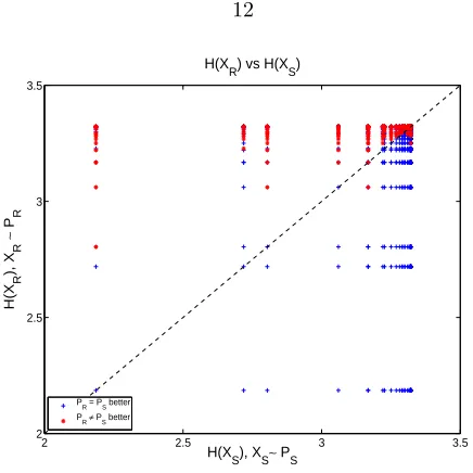
Figure 2.2 illustrates the entropy of different distributions. We plotH(XR) versusH(XS), where

H(·) is the entropy of the discretized probability distributions andXR∼PS and XS ∼PS, marking

the cases where usingPS 6=PR resulted in better out-of-sample performance of the algorithm. As it

is clear from the plot, these cases occur whenH(XS)< H(XR).

A simple way to think of the problem is to see that if we could freely choose a test distribution, and our learning algorithm outputsθ∗ as the learned parameters that minimizes some loss function

l(x, y, θ) on a training data set R = {(xi, yi)}, then to minimize the out-of-sample error we would

choosePS(x) =δ(x−x?), whereδis the delta-dirac function andx?= arg min

R (l(x, y, θ

∗_{))), the point}

in the input space where the minimum out-of-sample error occurs.

Similar results as those shown in Figure 2.1 are found whenNR= 300.

2.1.2 Fixing the test distribution

Figure 2.3 shows the result of the simulation in the other direction. Each entry in the matrix again corresponds to a pair of distributions PR and PS. However, this time we fix PS and evaluate the

percentage of runs where using PR 6=PS yields better out-of-sample performance than ifPR =PS.

(21)

2 2.5 3 3.5 2

2.5 3 3.5

H(X

R) vs H(XS)

H(X

S), XS∼ PS

H(X

R

), X

R

∼

P

R

PR = PS better

[image:21.612.194.412.68.286.2]

PR≠ PS better

Figure 2.2: H(XR) vs H(XS): Characterization of why out-of-sample performance is better if there

is a mismatch in distributions whenPR is fixed, using entropy.

This is the case that occurs in practice, where the distribution the system will be tested on is fixed by the problem statement. However, the training set might have been generated with a different distribution, and we would like to determine if training with a data set coming fromPS would have

resulted in better out-of-sample performance. If the answer is yes, then one can consider the matching algorithms that we mentioned to transform the training set into what would have been generated using the alternate distribution.

The simulation result is quite surprising, as once againthere is a significant number of entries where

more than 50% of the runs have better performance when mismatched distributions are used. For 14%

of the entries, a mismatch betweenPR and PS results in lower out-of-sample error, as indicated by

the light green, yellow, orange, and red entries in the matrix.

In this case, although the block structure is still present, there is no longer a clear pattern relating the entropies of the training and test distributions that allows explaining the result easily as in the previous simulation. Notice that there are cases where the mismatch is better if we choosePRof both

lower and higher entropy than the givenPS. This is clear in the plot since the indicated regions in

(22)

P_S PR

E

R,R’[I[Ex,f[Eout(x,R)] < Ex,f[Eout(x,R’)]]] (14.0% cases where this is majority)

Uniform Gaussians Exponentials 2−MG Uniform

Gaussians

Exp.

2−MG

0 0.1 0.2 0.3 0.4 0.5 0.6 0.7 0.8 0.9 1

Figure 2.3: Summary of Monte Carlo Simulation. Plot indicates, for each combination of probability distributions,_ER∼PR,R0∼PS[I[Ef,x∼PS[Eout(x, R, f)]<Ef,x∼PS[Eout(x, R

0_{, f}_)]]].

2.2 Empirical and analytic results in the regression setting

We have shown empirical evidence that a mismatch in distributions can lead to better out-of-sample performance in the classification setting, and now we focus on the regression setting to cover the other major class of learning problems. In this section, we use the expressions for the expected out-of-sample error as a function ofx, a general test point in the input spaceX, andR, the training set, averaging over target functions and noise realizations. These expressions are derived in detail in Appendix A, for the case where we use a squared loss function and a linear model with non-linear transformations for the hypothesis set. This correspond to the choice of linear model and loss function of the simulations shown in the previous section.

The difference now is that although we choose againX = [−1,1], in the regression settingY =_R. To analyze the most general regression case, we also introduce both “stochastic” and “deterministic” noise [2]. We takeyi =f(xi)+i, whereirepresents the stochastic noise, and wherefis more complex

than the elements ofH, sof /∈ H, hence the deterministic noise. We make the usual assumption about the stochastic noise, which is that it has zero mean and is iid. That is,E[] = 0, and E[T] =σN2I,

where I is the identity matrix and σN is the standard deviation of the noise. We also make the

assumption that the coefficients of the target function that are not included in the model,θC, have

covariance matrixE[θCθTC] =σ

2

(23)

As introduced in Appendix A, for simplicity we let

z=φ(x). (2.6)

We reorganize the features inz and elements ofθas

zT = [zT_M z_CT], θT = [θT_M θT_C] (2.7)

so that the firstM features ofz correspond to the features in the linear transformation that Hcan express. The matrixZ is the “transformed data matrix”, with

Z = [ZM ZC]T. (2.8)

These matrices are precisely defined in Appendix A.

Taking the expected value with respect to the noise, the out-of-sample error at a point x∈ X is given by

Ef,[Eout(x, R, f, )] =σC2kzCT −zTMZ †

MZCk2+σ2NzMT(ZMT ZM)−1zM+σ2N (2.9)

Notice that the above expression is independent of θ (i.e., the target function), as well as of the noise. The only remaining randomness in the expression comes from generatingR, and fromz, the point chosen to test the error, making the analysis very general.

Now, we are interested in minimizing the expected out-of-sample error. LetR denote a training data set generated according to PR, while R0 a data set generated according to PS. Can we find

PR6=PS such that

ER,x,θC,[Eout(x, R, f, )]<ER0,x,θC[Eout(x, R

0_{, f,}_)]? _(2.10)

The simulation shown in Section 2.1.2, although in a classification setting, suggests that this is the case. We run the same Monte Carlo simulation in this regression setting. The advantage is that the closed-form expression in Equation 2.9 already averages over target functions and noise, allowing us to run in a shorter time more combinations ofPRandPS. This expression only requires running Monte

Carlo simulations for the matrixZ and hence the two terms involving it,Z_M† ZC an (ZMT ZM)−1. The

expectation overx∼PScan be done using numerical integration, which is faster than the Monte Carlo

simulation in this one-dimensional setting. In this case, we consider the same families of distributions, but we vary the standard deviation of the distribution in smaller steps to obtain a finer grid.

(24)

P

S

PR

E

R,R’[I[Ex,θ

c,ε

[Eout(x,R)] < E

x,θ

c,ε

[Eout(x,R’)], for σ_N = σ_C = 0.2, M = 11, C = 21

Uniform Gaussians Exponentials 2−MG

Uniform

Gaussians

Exp.

2−MG

0 0.1 0.2 0.3 0.4 0.5 0.6 0.7 0.8 0.9 1

Figure 2.4: Monte Carlo simulation forER∼PR,R0∼PS[I[(Ex,θC,[Eout(x, R, θ, )]<Ex,θC,[Eout(x, R

0_{, θ,}_)]]],

M = 11,C= 21,N = 500, and σN =σC= 0.2.

for the non-linear transformation up to order 5, so thatM = 11. That is,

φM(x) = [1 cos(πx) sin(πx) · · · cos(5πx) sin(5πx)]T. (2.11)

On the other hand, the target functions were generated using harmonics up to order 10, so that

C = 21, with random Fourier coefficients. Both σC = σN = 0.2, and N = 500. Each entry in the

matrix computes

ER∼PR,R0∼PS[I[(Ex,θ,[Eout(x, R, θ, )]<Ex,θ,[Eout(x, R

0_{, θ,}_)]]]_, _(2.12)

which is the same quantity as that of Equation 2.5, except that nowf is determined byθ.

Notice that, as shown in Figure 2.3, the cases where mismatched distributions outperform matched ones cannot be explained using an entropy argument, as was the case in Section 2.1.1. Notice also that there are now combinations forPRandPS where almost 100% of the simulations returned lower

out-of-sample error for mismatched distributions. In particular, this happened whenPS was a truncated

Gaussian with small standard deviation (σ = 0.2), and when PS was a mixture of two Gaussians

withσ= 0.2. In addition, we note the similarity between this simulation and the one shown for the classification setting in Figure 2.3.

(25)

theN = 500 case. ForN = 100, the percentage is even higher, at 30%. Hence, there is clear evidence that although the number of combinations of distributions for which a mismatch between training and test distributions is larger for smallerN, the result still holds as N grows. Notice that in the simulations, the target function has 21 parameters. Hence, roughly forN = 100 there are effectively 5 samples per parameter, while forN = 3000 there are 150 samples per parameter. This covers a wide range, from small to large sample sizes, given the complexity of the target function.

Going back to the derived expressions, a closed-form solution for the expected out-of-sample error is given by

E[Eout(x, R, θ, )] =ER

Z ∞

−∞

σ_C2kz_CT−zT_MZ_M† ZCk2PS(x)dx+

Z ∞

−∞

σ2_Nz_MT(Z_MTZM)−1zMPS(x)dx+σ2N.

(2.13) It cannot be further reduced analytically due to the inverse matrix terms. Yet, if we assumeC=M

so that only stochastic noise is present, the expression reduces to

E,R,x,θ[Eout(x, R, θ, )] =σN2 +ER

Z ∞

−∞

σ_N2zT(ZTZ)−1zPS(x)dx

≥σ_N2

1 +

Z ∞

−∞

zT(_ER[ZTZ])−1zPS(x)dx

, (2.14)

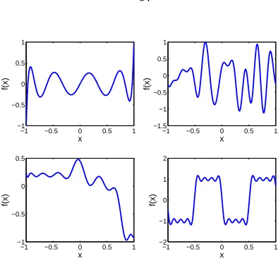
where we use the result in [37] for the expected value of the inverse of a matrix. With this expression, we can find a specific example of a mismatched training distribution that leads to better out-of-sample results. Again, without loss of generality, we pick the linear transformation consisting of Fourier harmonics, namely

z= [1 cos(πx) sin(πx) · · · cos(mπx) sin(mπx)]T (2.15)

as this allows a vast representation of target functions. Here,M = 2m+ 1. A few examples of the variety of the target functions that can be achieved with this model are shown in Figure 2.5.

IfPR is a Uniform distribution overX, or a Gaussian distribution truncated to this interval, then

ER[ZTZ] = ER

N

X

i=1

ziziT

= Ndiag(1,0.5,0.5, . . . ,0.5) (2.16)

(26)

−1 −0.5 0 0.5 1 −1 −0.5 0 0.5 1 x f(x)

−1 −0.5 0 0.5 1 −1.5 −1 −0.5 0 0.5 1 x f(x)

−1 −0.5 0 0.5 1 −1 −0.5 0 0.5 x f(x)

[image:26.612.203.400.75.263.2]

−1 −0.5 0 0.5 1 −2 −1 0 1 2 x f(x)

Figure 2.5: Sample realizations of targets generated with a truncated Fourier Series of 10 harmonics.

integration for the truncated Gaussians. This implies that

E,R,x,θ[Eout(x, R, θ, )] ≥ σN2

1 +_Ex

₂_m_{+ 1}

N

= σ_N2

1 +M

N

(2.17)

Now instead, pickRto be distributed according to Uniform[−a, a]. In this case,

ER[ZTZ]ij=

                                      

sinc(ja) ifi= 1, j is even sinc(ia) ifj= 1, iis even 1/2 1 + (−1)i_sinc(_ia₎

ifi=j6= 1 1/2 (sinc((i+j)a) + ifi6=j,and

sinc((i−j)a) iandj odd 1/2(sinc ((i+j)a)− ifi6=j,and sinc((i−j)a) iandj even

0 else

(2.18)

Figure 2.6 shows the closed-form bound for various choices of aand M = 10, choosing PS to be

a truncated Gaussian withσ = 0.4. The dotted line shows the bound for the case PR =PS. As it

is clear from the plot, there are various choices foraso that equation 2.10 is satisfied in terms of the bound.

(27)

0.9 0.95 1 1.05 1.1 1.15 0.04

0.045 0.05 0.055

a, where P

R = Uniform[−a,a]

Lower Bound for E

D,x,

ε

[E

o

ut]/

σn

2

P

R=U[−a,a],PS = N

*_{(0, 0.4}2₎

P

R=PS=N

[image:27.612.201.397.77.256.2]

*_{(0, 0.4}2₎

Figure 2.6: Bound forER,x,[Eout(x, R)]−σN2 whenRis generated with PR=PS =N∗(0,0.42) and

forPR6=PS withPR= Uniform[−a, a].

cases considered: we choosePS =N∗(0,0.42) and generateR0 according toPS, while Ris generated

according to U[−0.97,0.97]. Notice that we use a = 0.97 as this choice results in the lowest error bound from Figure 2.6. Usingm= 10,N = 500 and averaging over 108 _{realizations of}_R _and_R0 _we

obtain

ER,x,θ,[Eout(x, R, θ, )] = 1.0429σ2N < ER0_,x,θ,[E_out(x, R0, θ, )] = 1.0440σ2_N (2.19)

Hence, we have a concrete example of a distribution PR that is different from PS (Figure 2.7) that

(28)

−1 −0.8 −0.6 −0.4 −0.2 0 0.2 0.4 0.6 0.8 1 0

0.002 0.004 0.006 0.008 0.01 0.012

x

Density

P

S

P

[image:28.612.207.396.290.444.2]

R

Figure 2.7: Pair of distributions PR 6= PS such that expected out-of-sample error is lower when R

(29)

Chapter 3

The dual distribution

As shown in the previous chapter, contrary to the common presumption, the optimal distribution from which to sample training data is not necessarily the test distributionPS. Instead, we call the optimal

training distribution the dual distribution. This distribution only depends on the test distribution and not in the particular target function in question. In this chapter, we define the dual distribution precisely and then show how to obtain it in the general case, as well as in a practical scenario. We end the chapter with a comparison of the dual distribution approach and a related concept in active learning.

Given a distributionPS, we define adual distribution PR? to be a distribution that achieves

min

PR

ER,x,f,[Eout(x, R, f, )] (3.1)

where R is a data set generated according toPR andx∼PS. The above minimization problem of

course has the constraint thatPRmust be non-negative and should be normalized, so that the solution

yields a valid probability distribution.

3.1 Discrete input spaces

We first find the dual distribution in the case where the input space X is a discrete set. Let X =

{xj}dj=1, so that PR and PS become probability mass functions ondpoints. Hence, in this setting,

finding the dual distribution becomes an optimization problem ind−1 dimensions. We only optimize with respect tod−1 elements ofPR, since the last element can be determined from the normalization

constraint.

(30)

toPS, the noise, and the target function as

Ex,,θ[Eout(x, R, , θ)] =σ2N d

X

i=1

zT_i (ZTZ)−1ziPS(xi). (3.2)

In this case, there arePN

i=1

d i

possible data sets of sizeN (allowing for repetition of points in the data set) that could be obtained for any given PR. To simplify the notation, since X is finite, we

assign each of the points a number, from 1 tod, and we denote the out-of-sample error for each of these data sets as Ei1,i2,···,iN, where ik indicates the element number in X that corresponds to the

k’th data point inR.

Hence, we can find the expected out-of-sample error with respect toPR as

ER,x,,θ[Eout(x, R, , θ)] =

X

i1,i2,...,iN

pi1pi2· · ·piNEi1,i2,...,iN, (3.3)

where all theEi1,...,iN can be found using Equation 3.2. Therefore,P ?

R is the solution to the following

optimization problem:

min

p1,p2,...,pd

X

i1,i2,...,iN

pi1pi2· · ·piNEi1,i2,...,iN (3.4)

subject to

d

X

i=1

pi= 1

pi≥0

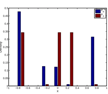
Let us look at a concrete example, withN = 3,

z= Φ(x) = [cos(πx) sin(πx)]T (3.5)

X = {−3/4,−1/4,0,1/4,3/4}

PS = [1/3,0,1/3,1/3,0]

[x1, x2, x3, x4, x5] = [−3/4,−1/4,0,1/4,3/4]

Solving the optimization problem given in Equation 3.4 yieldsP?

R6=PS, with

(31)

−1 −0.8 −0.6 −0.4 −0.2 0 0.2 0.4 0.6 0.8 1 0

0.05 0.1 0.15 0.2 0.25 0.3 0.35 0.4 0.45 0.5

x

Density

P

R*

[image:31.612.210.397.90.254.2]

P_S

Figure 3.1: Probability mass functions for a givenPS and its dual PR?, in a regression problem with

stochastic noise, discrete input spaceX ={−3/4,−1/4,0,1/4,3/4}, andN = 3.

For this example,

ER,x,,θ[Eout(x, R, θ, )] = 1.1391σ2n<ER0_,x,,θ[E_out(x, R, θ, )] = 1.5778σ2_n, (3.7)

where R0 is generated according to PS and R according toPR?. Clearly there is a gain by training

with the dual distribution, in this case. When running the optimization, for data sets that have repeated points that result in undefined out-of-sample error as the matrix (ZTZ)−1 is singular, we conservatively take their error to be the maximum finite out-of-sample error over all combinations of possible data sets. Figure 3.1 shows the dual distribution found, along with the givenPS.

Notice that if a different loss function is chosen and no closed form solution exists forEout(x, R),

the dual distribution can still be found using the same procedure as above. The only difference is thatEout(x, R) must be estimated, using a held-out set for instance, for each possible datasetR, so

that the correspondingEi1,...,iN can be computed and given as inputs to the optimization problem of Equation 3.4

A very important property of the optimization problem formulated in Equation 3.4 is that it is a convex optimization program. In fact it is a Geometric Program, although different from a standard Geometric Program, since the equality constraint is not a monomial. Yet, the problem is still convex. To illustrate this, let

ψi = log(pi) (3.8)

(32)

This change of variables implicitly makespi >0 so that the inequality constraints can be removed.

Also, the problem can be rewritten as

min

ψ1,ψ2,...,ψd

X

i1,i2,...,iN

ePNk=1ψik+Λi1,i2,...,iN _(3.10)

subject to

d

X

i=1

eψ_i = 1

(3.11)

Notice that the objective function is a sum of exponential functions of affine functions of ψi. Since

exponential functions are convex, affine transformations of convex functions are also convex, and sums of convex functions result in a convex function, the objective in Equation 3.10 is convex [19]. Following the same argument, the equality constraint is also convex, so that the optimization problem is a convex program.

Hence, if a minimum is found, this is the global optimum with a corresponding dual distribution. This problem can be solved with any convex optimization package. Furthermore, in most applications,

PS is generally unknown and is estimated by binning the data, which leads to a discrete version ofPS.

Therefore, this discrete formulation is appropriate to find dual distributions in such settings. Solving the Geometric Program described by Equation 3.10 thus allows us to find the dual distribution in various practical settings.

Nevertheless, we need to address the more general case of continuous input spaces. The following section describes how to find the dual distribution in that case, as well as how to implement it in a practical scenario.

3.2 The continuous case

When the input spaceX is continuous, as it is the case in most applications, the optimization prob-lem in Equation 3.1 is a functional optimization probprob-lem, since we are interested in finding the full distributionPR. We denote the corresponding probability density function bypR, and optimize with

respect to this density. The objective function of the optimization problem can be written as the functionalJ :P →R

J(p) =

Z

xN

· · ·

Z

x1

L(x1, . . . , xN) N

Y

i=1

p(xi)dx1· · ·dxN, (3.12)

where

(33)

and P is the set of all probability density functions with P ⊂ L1_{. (Recall an} _Lp _{space over} _X _is

defined as the space of functions f for which R

X|f(x)|

p _< _∞_{. Since probability density functions}

integrate to unity, they are elements ofL1_{). In the following subsection, we use functional calculus to}

arrive at the analytic condition that the dual distribution must satisfy.

3.2.1 Analytic condition for the dual distribution

To minimize the functionalJ(p), we first transform the variables, as we did in Section 3.1. Let

ψ(x) = logp(x) (3.14)

Λ(x1, . . . , xN) = log(L(x1, . . . , xN)). (3.15)

The optimization problem becomes

min

ψ =J(ψ) (3.16)

subject to

Z

eψ(x)dx= 1

where

J(ψ) =

Z

xN

· · ·

Z

x1

eΛ(x1,...,xN))+PNi=1ψ(xi)_dx

1· · ·dxN, (3.17)

and where the positivity constraints are implicit, given the domain of the logarithm. Now, recall that the gradient of a functionalJ(ψ), denoted as∇ψJ, is given by [28]

J(ψ+δζ) =J(ψ) +δh∇ψJ, ζi+O(δ2), (3.18)

whereδ∈R, δ >0, andζ∈ P is an arbitrary function. Consider the Lagrangian

L(ψ) =J(ψ) +λ

Z

eψ(x)dx−1

. (3.19)

Then, the dual distribution must satisfy

∇ψ(L(ψ(x))) = 0. (3.20)

In fact, we can use the Euler-Lagrange theorem [30] to show that if there is a function ψ that satisfies Equation 3.20, then it is the global minimizer. The theorem states that for a functionf ∈ C2_,

(34)

the functional

inf

X

I(u) = inf

X

Z

X

f(x, u, u0)dx (3.21)

where _X={u∈ C1_{, u} _{: [}_{a, b}_]d _→

R,|u|∂1Ω =u0}, u0 are the boundary conditions, and X = [a, b]

d_,

then ifI(u) admits a minimizer ¯u∈ C2_{, then ¯}_u_{satisfies the Euler-Lagrange (EL) equation:}

X ∂

∂xi

∂

∂u0f(x,u¯(x),u¯

0₍_x₎₎₋ ∂

∂uf(x,u¯(x),u¯

0₍_x_{)) = 0}_. _(3.22)

Conversely, if ¯usatisfies the EL equation and the mappingM(u, u0)→f(x, u, u0) is convex for every

x∈[a, b]d_{, then ¯}_u_minimizes_I₍_u_).

In our case, u=ψ, andJ(ψ) =I(ψ). Also, in our case,u0 does not appear, so thatf(x, ψ, ψ0) =

f(x, ψ). Hence, having the gradient of the Lagrangian with respect toψ equal to 0 is equivalent to satisfying the EL equation. This is the necessary condition.

Now, we can show that it is in fact a sufficient condition by using the converse. Notice that in our case_X=P is a convex set, as convex combinations of density functions are also convex. Hence, all that remains to show is that the mappingM is convex, that is, show that for 0≤α≤1,α∈_R,

M(αψ+ (1−α)φ)< αM(ψ) + (1−α)M(φ). (3.23)

Substituting, we have in the left hand side,

eΛ(x1,...,xN)+αPiψ(xi)+(1−α)Piφ(xi)_. _(3.24)

On the right hand side we have

αeΛ(x1,...,xN)+Piψ(xi)_{+ (1}₋_α₎_eΛ(x1,...,xN)+Piφ(xi)_. _(3.25)

Now, we notice that due to the strict convexity of the exponential function

eαθ1+(1−α)θ2 _{< αe}θ1_{+ (1}₋_α₎_eθ2_. _(3.26)

Hence, dividing both sides of Equation 3.23 by eΛ(x1,...,xN) _{and substituting} _θ

1 = Piψ(xi) and

θ2=Piφ(xi) shows that the mappingM is strictly convex.

(35)

We now compute the gradient of the Lagrangian. For simplicity, let dR denotedx1· · ·dxN, and

letRdenote the support of the set{x1, . . . , xN}then

J(ψ+δξ) =

Z

R

ePNi=1ψ(xi)+δξ(xi)+Λ(x1,...,xN)_dR

=

Z

R

ePNi=1ψ(xi)+Λ(x1,...,xN) _{1 +}_δ N

X

i=1

ξ(xi) +O(δ2)

!

dR

=J(ψ) +δ

Z

R

ePNi=1ψ(xi)+Λ(x1,...,xN) N

X

i=1

ξ(xi)dR

=J(ψ) +

N

X

i=1

Z

xn,n6=i

ePNi=1ψ(xi)+Λ(x1,...,xN)_dx

nn6=i, ξ(xi)

, (3.27)

where the simplification follows from using a Taylor expansion of the exponential. Finally, since the loss functions we are interested in are independent of the order of the points in the training set, then the logarithm of the loss function Λ(x1, . . . , xN) is symmetric with respect toxi. Therefore,

∇ψ(J(ψ(xn))) =NExi∼eψ i6=n

[L(x1, . . . , xN)]. (3.28)

Following a similar procedure for the second term in the Lagrangian, we obtain that at pointxn

∇ψ(L(ψ(xn)) = NExi∼eψ i6=n

[L(x1, . . . , xN)] +λ

!

eψ(xn) _(3.29)

We can now use the constraint to findλby integrating the above equation overxn. We obtain

λ=−N eψ(xn)

E xi∼p

i=1,...,N[L(x1, . . . , xN)] (3.30)

Substituting forλwe obtain the optimality condition that the dual distribution needs to satisfy:

p(xn)

Exi∼p

i6=n[L(x1, . . . , xN)]−E xi∼p

i=1,...,N[L(x1, . . . , xN)]

= 0. (3.31)

This condition applies to the dual distribution in the general case, without making assumptions about the target class or the learning model. Now, all that remains is to findpthat satisfies this condition, which can be done, for example, using functional gradient descent [49].

The functional gradient descent step is given by

(36)

whereη is the learning rate, hence

p(xn) :=p(xn)−ηN

Exi∼p i6=n

[L(x1, . . . , xN)]−E xi∼p i=1,...,N

[L(x1, . . . , xN)]

p(xn). (3.33)

Notice that the integral of the update over xn is 0. Hence, this update guarantees that the

nor-malization constraint is satisfied at each step, so that gradient descent works in this case as in an unconstrained problem. Therefore, if the initial condition is a valid probability density function (pdf), all subsequentp’s will also be valid pdf’s.

The interpretation of this update is very intuitive: If a pointxn is included in the training set,

and the resulting out-of-sample error is lower than the expected out-of-sample error withN points, that is_Exi∼p

i6=n[L(x1, . . . , xN)]<E xi∼p

i=1,...,N[L(x1, . . . , xN)], then p(xn) should be increased. If including

the point leads to a higher out-of-sample error, then the density at this point should be decreased. In the following subsection, we introduce a concrete example of how the condition of Equation 3.31 can be used computationally to derive the dual distribution.

3.2.2 Dual distribution examples

As shown in the previous subsection, finding the dual distribution reduces to performing functional gradient descent. However, the update rule depends on being able to compute the expected out-of-sample error Exi∼p

i6=n[L(x1, . . . , xN)]. Computing the expected value with respect to the training set

can be readily done using Monte Carlo (MC) simulation. This can be slow unless a closed form for

L(x1, . . . , xN) exists.

If a squared loss function is used for `, and the hypothesis class H is chosen to be a linear model (which can include non-linear transformations of the inputs), then a closed-form solution for

L(x1, . . . , xN) exists. This solution is independent of the specific target function. Hence, in this

setting, the dual distribution can readily be found. The closed-form solution, as derived in Appendix A is given by

L(x1, . . . , xN) =σC2kφC(x)T −φM(x)TΦ−_{M M}1 ΦM Ck2+Ex∼PS

σ2_NφM(x)TΦ_{M M}−1 φM(x)+σN2, (3.34)

whereφ:X → ZM+C _{denotes the transformation of the input, with}

φ(x) = [φM(x)T φC(x)T]T, (3.35)

so thatφM :X → ZM represents the part of the target function that can be captured by the model,

(37)

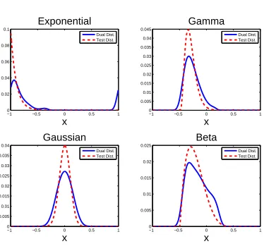
−10 −0.5 0 0.5 1 0.005 0.01 0.015 0.02 0.025 0.03 0.035 0.04 Gaussian x Dual Dist. Test Dist.

−1 −0.5 0 0.5 1 0 0.005 0.01 0.015 0.02 0.025 Beta x Dual Dist. Test Dist. −10 −0.5 0 0.5 1

0.02 0.04 0.06 0.08 0.1 Exponential x Dual Dist. Test Dist.

−1 −0.5 0 0.5 1 0 0.005 0.01 0.015 0.02 0.025 0.03 0.035 0.04 0.045 Gamma x Dual Dist. Test Dist.

Figure 3.2: Examples of dual distributions, for 1-D test distributions, in a linear regression problem.

Table 3.1: Out-of-sample (OoS) performance improvement when training the learning algorithm with data coming from the dual distribution rather than from the test distribution

Test Parameters OoS error

Distr. improvement

Exponential λ= 5 46.3%

Gamma α= 4,β= 0.05 32.0%

Gaussian µ= 0, σ= 0.1 21.4%

Beta α= 2,β= 5 10.0%

F ν1= 100,ν2= 80 5.7%

Weibull λ= 1, k= 5 2.2%

Uniform [-1,1] 0.5%

2-D Gaussian Σ = [0.12 0.08; 0.08 0.12] 22.6%

2-D MG Σ = [0.12 0.06; 0.06 0.12] 5.71%

ΦM M ∈ ZM×M and ΦM C ∈ ZM×C defined for the training input pointsx1, . . . , xN are given by

ΦM M = ZMTZM = N

X

i=1

φM(xi)φM(xi)T, (3.36)

ΦM C = ZMTZC= N

X

i=1

φM(xi)φC(xi)T. (3.37)

Finallyσ2

N andσ2C characterize the energy of the stochastic noise and ‘excess’ target complexity as

[image:37.612.214.401.86.264.2]

explained before.

(38)

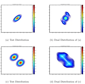
Test Distribution. Error: 0.0030781

−1 −0.8 −0.6 −0.4 −0.2 0 0.2 0.4 0.6 0.8

−1 −0.8 −0.6 −0.4 −0.2 0 0.2 0.4 0.6 0.8 0 0.01 0.02 0.03 0.04 0.05

(a) Test Distribution

Dual Distribution. Error: 0.0023812

−1 −0.8 −0.6 −0.4 −0.2 0 0.2 0.4 0.6 0.8

−1 −0.8 −0.6 −0.4 −0.2 0 0.2 0.4 0.6 0.8 0 0.01 0.02 0.03 0.04 0.05

(b) Dual Distribution of (a)

Test Distribution. Error: 0.0035724

−1 −0.8 −0.6 −0.4 −0.2 0 0.2 0.4 0.6 0.8

−1 −0.8 −0.6 −0.4 −0.2 0 0.2 0.4 0.6 0.8 0 0.002 0.004 0.006 0.008 0.01 0.012 0.014 0.016 0.018 0.02

(c) Test Distribution

Dual Distribution. Error: 0.0033135

−1 −0.8 −0.6 −0.4 −0.2 0 0.2 0.4 0.6 0.8

−1 −0.8 −0.6 −0.4 −0.2 0 0.2 0.4 0.6 0.8 0 0.002 0.004 0.006 0.008 0.01 0.012 0.014 0.016 0.018 0.02

[image:38.612.169.451.82.361.2]

(d) Dual Distribution of (c)

Figure 3.3: Examples of dual distribution, for 2-D test distributions. (a) 2-D Gaussian; (b) Dual distribution for (a); (c) Mixture of 2-D Gaussians; (d) Dual distribution for (c).

the model. The simulation parameters were set toN = 100, M = 3, C = 5, σN =σC = 0.2. The

input domain isX = [−1,1], so the distributions were zeroed out outside this domain and renormal-ized. Table 3.1 shows the parameters of the test distributions and also indicates the improvement in out-of-sample performance when the learning algorithm is trained with samples coming from the dual distribution, rather than from the test distribution. Figure 3.3 shows the dual distribution for two-dimensional test distributions.

As it is clear from Table 3.1, the gains in using the dual distribution can be significant. For these examples,N was chosen so that there were enough samples to estimate the three parameters in the model (M = 3), and the target was more complex than the model.

The reader may be wondering how the sample size (N), the excess target complexity with respect to the model (C−M) and its magnitude (σC), and the stochastic noise level (σN) affect the dual

distribution. We address this question in the following section.

3.3 Variability of the dual distribution

(39)

the change in dual distribution due to these factors.

3.3.1 Asymptotic behavior

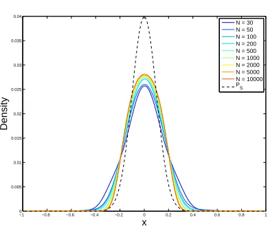
The first factor we analyze is the dependence of the dual distribution onN, the training set sample size. In particular, consider the case whereN→ ∞. Recall that the dual distribution is the distributionP

that minimizes the quantityExi∼P[L(x1, . . . , xN)]. Using the closed-form expression forL(x1, . . . , xN) in the squared loss and linear model with non-linear transformations case, we can separate the impact of the stochastic and deterministic noise terms. The stochastic term, that is, the term proportional toσ_N2 from Equation 3.34, isO(1/N). Notice that:

Exi∼P

Φ−_{M M}1

= 1

NExi

  1 N N X i=1

φM(xi)φM(xi)T

!−1 

AsN→ ∞,

1

N

X

i=1

φM(xi)φM(xi)T P

−→_Exi∼P[φM(xi)φM(xi)

T_] _(3.38)

where−P→denotes convergence in probability. Substituting, the stochastic noise term simplifies to

1

NEx

h

σN2φM(x)TExi

φM(xi)φM(xi)T

−1

φM(x)

i

. (3.39)

Therefore, this term vanishes asN → ∞.

The remaining term, on the other hand, is O(1), so this is the term that must be minimized. Following a similar analysis as above, it follows that

lim

N→∞Exi∼P[L(x1, . . . , xN)] =σ

2

N +σ

2

CExkφC(x)T −φM(x)TΦk2, (3.40)

where

Φ = _Exi

φM(xi)φM(xi)T

−1

Exi

φM(xi)φC(xi)T

. (3.41)

Notice that if the collection of features {φi(x)}iM=1+C (the components ofφ(x)) form an orthonormal

set underP, then by definition

Exi∼P[φi(x)φj(x)] =

 



1 ifi=j

0 ifi6=j

. (3.42)

Therefore,Exi

φM(xi)φM(xi)T

=I, andExi

φM(xi)φC(xi)T

(40)

−10 −0.8 −0.6 −0.4 −0.2 0 0.2 0.4 0.6 0.8 1 0.005

0.01 0.015 0.02 0.025 0.03 0.035 0.04

x

Density

N = 30 N = 50 N = 100 N = 200 N = 500 N = 1000 N = 2000 N = 5000 N = 10000 P

[image:40.612.205.400.93.261.2]

S

Figure 3.4: Example Dual Distributions in 1-Dimension when the training set sizeN changes, for

PS = N(0,0.12), M = 3, C = 5, using a linear model with Fourier harmonics and a squared loss

function.

polynomials, or whenPis a uniform distribution and the features are Fourier harmonics, among other cases. In this case, the error would reduce toσ2

N +Cσ2C, and hence there would be no dependence of

the error on the training distribution.

However, when the features are not orthonormal under P, the out-of-sample error still changes with the training distribution in the limit asN → ∞. We can minimize Equation 3.40 with respect to Φ. This optimization problem is strictly convex, as it is a quadratic program in the entries of Φ. Finding the gradient and setting it to zero, we find that the necessary and sufficient condition for the minimum is to satisfy the equation

ΦTEx∼PS[φM(x)] =Ex∼PS[φC(x)]. (3.43)

The solution to this equation will depend on the type of features chosen. For example, if the features outside the model have mean zero, making the right hand side vanish, then the distributionP that makes the features orthogonal will be the solution.

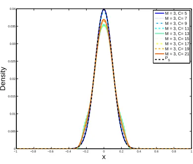
Figure 3.4 shows the effect ofN on the dual distribution in a specific example. For this example

PS =N(0,0.12),M = 3,C= 5,σN =σC = 0.2 andN varies. We used a linear model with Fourier

harmonics and a squared loss function. Notice that the variability of the dual distribution is small as

(41)

−10 −0.8 −0.6 −0.4 −0.2 0 0.2 0.4 0.6 0.8 1 0.005

0.01 0.015 0.02 0.025 0.03 0.035 0.04

x

Density

M = 3, C= 5 M = 3, C= 7 M = 3, C= 9 M = 3, C= 11 M = 3, C= 13 M = 3, C= 15 M = 3, C= 17 M = 3, C= 19 M = 3, C= 21 P

[image:41.612.205.400.96.262.2]

S

Figure 3.5: Example Dual Distributions in 1-Dimension when the deterministic noise changes, for

PS =N(0,0.12),N = 100, M = 3, using a linear model with Fourier harmonics and a squared loss

function.

3.3.2 Effect of noise and complexity

We now look at the effect of target complexity. Notice that as the target complexity grows, the deterministic noise term dominates L(x1, . . . , xN). Hence, although the stochastic noise term does

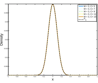
not vanish as it is the case when N → ∞, it is still the deterministic noise term that drives the minimization. Figure 3.5 shows the dual distributions for the same test distribution, as the target complexity increases. As the figure shows, there is little variability with respect to the change in target complexity. The variability actually disappears completely if Hermite polynomials are chosen for the features. In this case, for all values ofC,P? ₌_P

S, and Figure 3.6 exemplifies this behavior.

If we now look at the case where only stochastic noise is present in the data, we notice that for finiteN, the error becomes

σ_N2_Ex∼PS

φM(x)TExi∼P

Φ−_{M M}1

φM(x)

. (3.44)

Again we have a quadratic form, but this time in terms of the matrix ΦM M rather than in term of

the matrix Φ. This objective function has a minimum of zero, which is achieved at _E[ΦM M] = 0.

However, ΦM M follows the particular form defined in Equation 3.36, which constrains the quadratic

program so it yields a different solution.

Figure 3.7 illustrates the effect of increasing the stochastic noise in a concrete example, where the dual distribution is calculated for the same test distribution, andσN is increased while holding N,

(42)

−10 −0.8 −0.6 −0.4 −0.2 0 0.2 0.4 0.6 0.8 1 0.005

0.01 0.015 0.02 0.025 0.03 0.035 0.04

x

Density

M = 3, C= 5 M = 3, C= 7 M = 3, C= 9 M = 3, C= 11 M = 3, C= 13

[image:42.612.205.400.97.262.2]

P_S

Figure 3.6: Example Dual Distributions in 1-Dimension when the deterministic noise changes, for

PS = N(0,0.12), N = 100, M = 3, using a linear model with Hermite polynomial features and a

squared loss function.

As it can be seen from the above analysis, the dual distribution is fairly robust with respect to the different components of the learning problem. Namely, the sample size, the noise, and the target complexity. This property allows using the dual distribution in a practical setting where components like the level of noise and target complexity might not be exactly known. The following subsection describes how to find the dual distribution in a practical setting.

3.4 Using the dual distribution in a practical setting

The dual distribution can be applied in two different settings. The first is the population-based active learning setting. This is a special case of active learning, in which contrary to supervised learning where the training data set is fixed, it is possible to sample points according to a desired distribution. This active learning setting is common in applications of experiment design, where the idea is precisely to design the distribution from which points will be sampled. In this case, the design distribution plays the role of the dual distribution, and is chosen by searching within a class of distributions [63]. The second setting where the dual distribution can be used, is in the supervised learning setting case that we have been discussing. In this section, we will show how to use the dual distribution even though the data has already been generated using a fixed distribution. We describe in detail how to do this, and show results on benchmark datasets.

(43)

−10 −0.8 −0.6 −0.4 −0.2 0 0.2 0.4 0.6 0.8 1 0.005

0.01 0.015 0.02 0.025 0.03 0.035 0.04

x

Density

σ_N = 0

σ_N = 0.1

σ_N = 0.2

σ_N = 0.4

σ_N = 1

σ_N = 2

σ_N = 5

[image:43.612.205.400.95.262.2]

P_S

Figure 3.7: Example Dual Distributions in 1-Dimension when the stochastic noise changes, forPS = N(0,0.12_),_N _{= 100,}_M _{= 3,}_C_{= 5, using a linear model with Fourier harmonics and a squared loss}

function.

First, the data set is fixed, so the expected values in Equation 3.33, which are taken with respect to data set generations, cannot be evaluated. Hence, there is a problem in computing the dual distribution itself. The second problem is how to use the dual distribution, since the data is already fixed. It is now necessary to make the data set appear as if it came from a different distribution. Here we describe how to approach both problems.

In order to get the dual distribution with only one data set sample, we make use of the fact that in this setting, the dual distribution only needs to be computed at the positions xi, i = 1, . . . , N.

The reason for this is that we will use matching algorithms to make the sample look as if it was distributed according to the dual distribution. As we explain shortly, matching algorithms only need to compute weights for each of the samples. Hence, it is no longer necessary to compute the full function, but simply its values atN locations. Also, we notice that the gradient at a pointxn is given

by the difference in the expected loss with respect toN−1 training points, havingxn present in the

training set, and the expected loss with respect toN training points (Equation 3.31). So, given that only one data set is available, E xi∼p

i=1,...,N[L(x1, . . . , xN)] is approximated by the estimate of the loss

using a single sample (i.e. a single data set). On the other hand,Exi∼p

i6=n[L(x1, . . . , xN)] is estimated

by increasing the weight of pointxn and finding the resulting loss. The difference of the two terms

will approximate the effect of this point on the loss, and hence determine an approximate value of the gradient at this point.

(44)

the covariate shift literature. These methods are described in Section 1.2. All these methods are variants of importance weighting [64], and their goal is to estimate the weightsw(x) =pS(x)/pR(x),

wherepRandpS are the training and test densities, respectively. They do this, in order to matchPR

toPS. Some of the methods, like KMM [38], KLIEP [67], and LSIF [42] usually perform better in the

covariate shift correction problem, as they try to estimate the ratio directly, rather than computing the numerator and denominator separately. This can be done when there are unlabeled samples available, coming from both the training and test distributions. In our case, the importance weights are given byw(x) =p?

R(x)/pR(x). Here, the numerator is found directly through functional gradient descent,

having no available samples distributed according to it. Hence, it is necessary to use methods that actually compute the training density pR. This can be done either by finding a histogram of the

training set with the adequate resolution, or using other non-parametric methods like Kernel Density Estimation (KDE) [56] and [53]. Chapter 5 proposes an alternative method that can be used to match the training distribution to any other distribution, such as the dual. We call this algorithm Soft Matching.

Therefore, the dual distribution can be used in the supervised learning setting, using the men-tioned approximation for the functional gradient descent, and making use of importance weighting to change the distribution of the training data. Table 3.2 shows the average out-of-sample error, in both classification and regression tasks on 17 benchmark datasets [7] and [68], when the training set is transformed so that it appears distributed as the dual distribution. The values are compared to the case where no changes are made to the training set.

The results are averaged over 1,000 different splits of the data into training and test sets. The training set is also split further, as a validation set is needed to compute the expected loss for the functional gradient descent. The reported errors are on the test set which is not used at all during training, nor during computation of the dual distribution. For all datasets 25% of the data was left aside for testing, 25% was part of the validation set, and the remaining 50% was used for training. For classification problems, weighted SVMs with Gaussian kernels were used, choosing the kernel width as in [38], with thelibsvm implementation [23]. Ridge regression was used for the remaining data sets, with regularization parameterλ= 0.1.

Optimal Data Distributions in Machine Learning

Optimal Data Distributions in Machine Learning

Carlos R. Gonz´

alez

Acknowledgements

Abstract

Contents

I

Optimal Data Distributions in Machine Learning

1

II

Behavior Analysis with Machine Learning

77

Part I

Optimal Data Distributions in

Chapter 1

Introduction

1.1

Overview

1.2

Literature overview

1.3

The learning setup

Chapter 2

Is it better to have

P

R

=

P

S

?

2.1

Empirical results in the classification setting

2.1.1

Fixing the training distribution

2.1.2

Fixing the test distribution

2.2

Empirical and analytic results in the regression setting

Chapter 3

The dual distribution

3.1

Discrete input spaces

3.2

The continuous case

3.2.1

Analytic condition for the dual distribution

3.2.2

Dual distribution examples

3.3

Variability of the dual distribution

3.3.1

Asymptotic behavior

3.3.2

Effect of noise and complexity

3.4

Using the dual distribution in a practical setting

_R

_S