Towards data driven magnetic materials discovery

Towards Data-Driven Magnetic

Materials Discovery

by

Mario ˇ

Zic

A thesis submitted in partial fulfillment for the degree of Doctor of Philosophy

in the

Trinity College Dublin School of Physics

I declare that this thesis has not been submitted as an exercise for a degree at this or

any other university and it is entirely my own work. I was involved in a number of

collaborations, and where it is appropriate my collaborators are acknowledged for their

contributions.

I agree to deposit this thesis in the University’s open access institutional repository

or allow the library to do so on my behalf, subject to Irish Copyright Legislation and

Trinity College Library conditions of use and acknowledgement.

Signed:

Date:

Abstract

Trinity College Dublin

School of Physics

Doctor of Philosophy

byMario ˇZic

Magnetic materials underpin many of the technologies that define the world we live in.

Despite the tremendous technological progress, the discovery of new magnetic materials

has been rather slow. In this Thesis we explore and develop new, data-oriented, methods

for the accelerated discovery and development of new magnetic materials. We utilize

available theoretical databases of Heusler alloy properties to: develop a high-throughput

(HT) screening procedure for the discovery of new permanent magnets, identify the

de-fects in Mn-Ru-Ga thin films, and build machine learning (ML) models for predicting

the structural and the magnetic properties of Heusler alloys. We identify a dozen

mate-rials, which meet all of the criteria for permanent magnet applications. The analysis of

the HT data allowed us to understand the ideal composition of hard magnetic materials

in the family of regular Heusler alloys, and to show how structure-property constraints

affect the abundance of the potential candidates for technological applications. We find

that hard permanent magnets occur with a frequency smaller than 1 in 10 000, with

respect to the overall population of the regular Heusler alloys in the database. We then

demonstrate that the ML techniques can be used both to improve the efficiency of the

HT procedure and to perform a data-driven investigation of the material properties. In

the case of the Mn-Ru-Ga thin films we show how the HT data can be utilized to guide

the modelling of technologically relevant materials. The HT data was used to

iden-tify the nature of the defects that occur in the films, and hence, to obtain an accurate

theoretical description of the material properties. We build ML models to investigate

the magnetism of Fe in Heusler alloys. We then study how the local chemical

environ-ment affects its magnetic moenviron-ment and thus address the structure-property relationship

directly. We also show that new knowledge about the physics of materials can be

ex-tracted directly from the data. This work clearly demonstrates the potential that ML

techniques have to offer in the analysis of a vast amount of materials data and paves the

I am in debt to a number of people who have helped me to realize this Thesis. First

and foremost, I would like to thank my supervisor Prof. Stefano Sanvito for providing

me the opportunity to do the PhD. in his group, for his guidance and trust, which has

allowed me much freedom in the research. I also thank him for patiently reading this

Thesis and providing valuable feedback. Many thanks are also due to Stefania Negro,

who has kindly helped me with many administrative and financial matters throughout

these four years.

This PhD. has been made an enjoyable experience by the members of the Computational

Spintronics group, past and present - thank you all. Many thanks go to Dr. Thomas

Archer, who has served as my co-supervisor, and has helped me a lot throughout the

PhD. I am particularly grateful for the companionship to: Dr. Rajarshi Tiwari, Filiberto

Biolcati Rinaldi, Mario Galante, Dr. Alessandro Lunghi, Dr. Carlo Motta, and Dr. Igor

Popov. Special thanks go to Dr. Jacopo Simoni and Emanuele Bosoni for their friendship.

I would like to thank my collaborators from the group of Prof. Mike Coey, especially

Dr. Karsten Rode. Working with him was both enjoyable and fruitful. I would also like

to thank Prof. Stefan Bl¨ugel, for hosting me in his group (Forschungszentrum J¨ulich,

Germany). I thank his group members: Dr. Daniel Wortmann, Dr. Marjana Leˇzai´c,

and Dr. Phivos Mavropoulos, for their hospitality and the professional advice. Special

thanks go to Phivos, to whom I am greatly indebted. I thank him for his time, his help,

and the computer codes, all of which he shared with me so generously. Without his help

a big part of this Thesis would not be possible.

I would like to thank my girlfriend, for the companionship, the support, and the patience

all these years. Finally, I would like to thank my family for the support and the sacrifices

which had allowed me to achieve all this. I hope I will be able to repay some of that

debt by making you proud.

This work would not be possible without the financial support from the FP7 project

“ROMEO” and Science Foundation of Ireland. The computational resources have been

provided by the Trinity Center for High Performance Computing (TCHPC) and by the

Irish Centre for High-End Computing (ICHEC).

The template for this Thesis can be found atwww.sunilpatel.co.uk.

Declaration of Authorship iii

Abstract iv

Acknowledgements v

List of Figures xi

List of Tables xvii

Introduction 1

1 Theoretical Background and Methods 7

1.1 The Electronic Structure Theory . . . 7

1.1.1 The Many-Body Problem . . . 9

1.1.2 The Density Functional Theory . . . 14

1.1.2.1 The Kohn-Sham Approach . . . 16

1.1.2.2 The Kohn-Sham Approach for Magnetic Systems . . . 18

1.1.2.3 Interpretation of the Kohn-Sham values . . . 22

1.1.2.4 Approximations of the Exchange Correlation Functional . 25 1.1.2.5 Pseudopotentials . . . 27

1.1.3 Electronic Structure of Solids . . . 29

1.1.3.1 Semi-Classical Theory of Electron Transport . . . 34

1.1.4 The Origin of Magnetism . . . 37

1.1.4.1 Application of SDFT to Magnetic Systems . . . 42

1.2 Machine Learning . . . 50

1.2.1 Statistical Learning Theory . . . 52

1.2.2 Bias-Variance Trade-Off and Over-Fitting . . . 55

1.2.3 Model Selection and the Error Estimation . . . 57

2 Accelerated Discovery of Permanent Magnets Using High-Throughput DFT Calculations 61 2.1 Introduction . . . 61

2.2 High-Throughput DFT Screening Approach for Permanent Magnet Dis-covery . . . 64

2.3 Material Selection . . . 67

2.4 TC Calculations . . . 68

2.4.1 Method . . . 68

2.4.2 Results . . . 70

2.5 MCA Calculations . . . 76

2.5.1 Method . . . 76

2.5.2 Results . . . 77

2.6 Discovering Hard Magnets Using a Machine Learning Classification . . . . 81

2.6.1 Method . . . 81

2.6.2 Results . . . 84

2.7 Conclusions . . . 88

3 Designing a Fully-Compensated Ferrimagnetic Half-Metal 91 3.1 Introduction . . . 91

3.2 Properties of Stoichiometric Mn2RuxGa Heusler Alloys . . . 95

3.3 Relative Stability of the Competing Mn-Ru-Ga Heusler Phases: a High-Throughput Approach . . . 104

3.4 The Effects of the Mn-Ga Substitution on the Properties of MRG Films . 107 3.5 Conclusions . . . 114

4 Magnetism of Iron in Heusler Alloys: a Machine Learning Approach 117 4.1 Introduction . . . 117

4.2 Method . . . 120

4.2.1 General Considerations . . . 120

4.2.1.1 Defining the problem . . . 121

4.2.1.2 Data Selection . . . 122

4.2.1.3 Building the Model . . . 124

4.2.1.4 Testing the Model . . . 126

4.2.1.5 Application . . . 127

4.2.2 Machine Learning Model for Magnetism . . . 128

4.2.2.1 Heusler Alloy Volume Regression Model . . . 130

4.2.2.2 Magnetic Moment Regression Model . . . 133

4.3 Results . . . 136

4.3.1 Role of the Coordination Shells . . . 136

4.3.1.1 Next-Nearest Neighbour . . . 137

4.3.1.2 Nearest Neighbour . . . 138

4.3.1.3 Physical Origin of the Magnetic Moment Trend . . . 140

4.3.2 Application . . . 142

4.4 Conclusions . . . 144

Conclusions 147

C Glossary 157

1 Simplified schematic of the computational high-throughput (HT) work-flow. First a set of preselected structures is passed to the automatized calculation engine, namely material properties are calculated and post-processed for storage into the database. In the final step the data in the database is subjected to the analysis. The results of the analysis may be the final objective of the HT calculation or just a new selection of struc-tures can be made and fed into the input of the HT cycle. The Roman numerals denote the three key steps of the HT search: I) virtual materials growth, II) rational data storage, and III) data analysis. . . 2 2 Crystal structure of the (X2Y Z) full Heusler alloys, also known as the

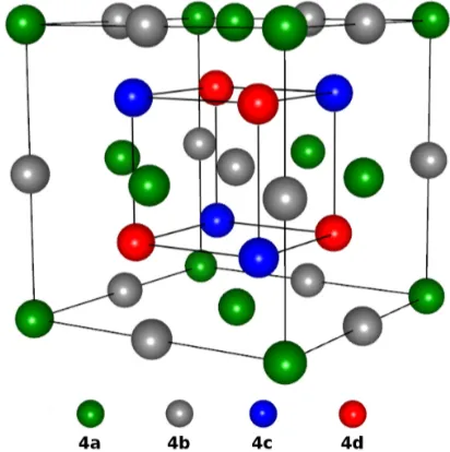
L21 phase. TheZ atom is typically a main group element, occupying the 4b site. The Y atom occupies the 4a site and the two X atoms occupy the 4c and 4d site. In the half-Heusler structure, C1b, the 4d site remains unoccupied. . . 4

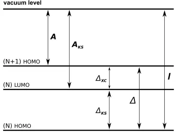
1.1 Flow chart of the self-consistent loop used to solve the system of Kohn-Sham (KS) equations (1.21). . . 18 1.2 Molecular level diagram illustrating the Kohn-Sham (KS) bandgap

prob-lem. The HOMO and the LUMO denote the highest occupied and the lowest unoccupied molecular orbital, respectively. The number of elec-trons in the system, N, is indicated in the brackets. The true ionization energy, I, and the affinity, A, are shown. Within the KS approach, the affinity, AKS, is determined by the KS bandgap, ∆KS. The latter

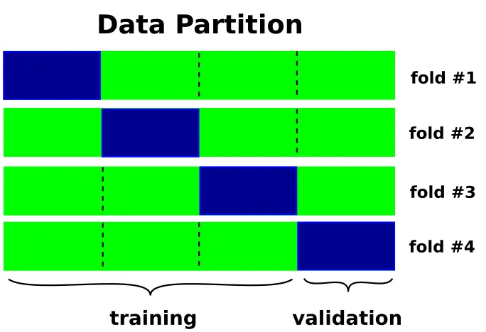
repre-sents a lower bound for the fundamental bandgap, ∆. . . 24 1.3 The four-fold cross-validation. The data is randomly distributed across

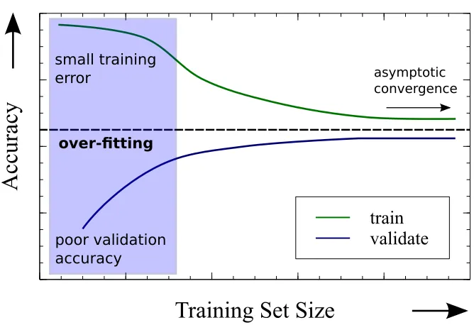
four bins of equal size. For each fold, three bins are used for the training (green) and one bin is used for the validation (blue). Four iterations are performed, each time selecting a different bin for the validation. The cross-validation error is obtained as an average error over the four folds. 58 1.4 Hypothetical learning curve plot. The training and the validation

accu-racy, green and blue curve respectively, are plotted as a function of the training set size. The over-fitting region is indicated by the shaded back-ground. For large training set size the asymptotic accuracy of a given model is achieved. Both curves converge to the same value. . . 60

2.1 Protocol for the high-throughput screening of permanent magnets. The procedure is broken down into three steps (I - III). We start from a full database of Heusler alloys [31]. The screening criteria are then applied, i.e. we look for stable magnetic materials with a tetragonal ground-state structure. This is illustrated as a two step data reduction. In the second step we calculate the Curie temperature,TC, for the candidate materials.

The materials with a TC <500 K are filtered out. Finally, we proceed by

calculating the magnetic anisotropy energy (MAE). . . 66 2.2 Schema of the automated KKR workflow. The user needs to provide the

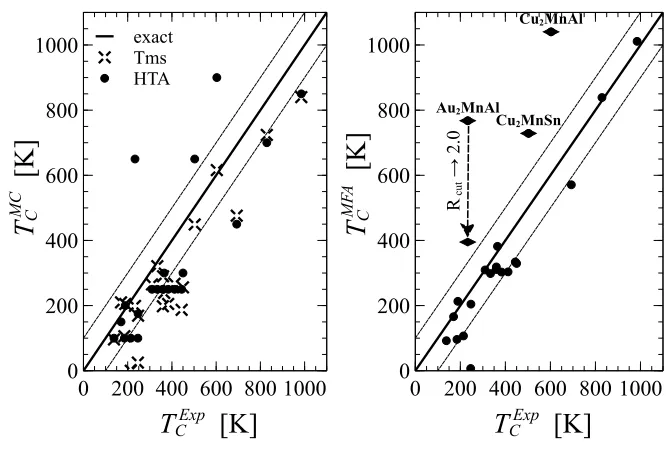
site occupation and the crystal structure data as an input. The workflow takes care of the rest. The ground state is obtained in two steps. First the magnetic moment is converged and then, in the second step, the electron density. Each of these steps is automatically restarted if convergence is not reached. Finally, the Monte Carlo (MC) input files are prepared and the mean-field approximation (MFA) Curie temperature, TC, is calculated. In case the ground state calculation fails, the error handler inspects the error and decides which recovery procedure to follow. Otherwise, the calculation is stopped. . . 69 2.3 Comparison of the Curie temperatures, TC, calculated using the KKR

workflow presented here (HTA).Left Panel -shows the Monte Carlo (MC) TC. The results obtained using the HTA are plotted against the corre-sponding data from the Tillmanns dataset (Tms) [144]. The line of the exact agreement and the±100 K error bar are indicated by the full and the dashed lines, respectively. Three of the materials show a poor agreement (diamonds), due to the truncation of theJij cutoff radius (cf. figure 2.4). Right Panel -compares the MC and the mean-field approximation (MFA) TC, calculated within the HTA. . . 72 2.4 Comparison of the calculated Curie temperatures, TC, and the

corre-sponding experimental data. Left Panel -comparison of the Monte Carlo (MC) TC, obtained using the KKR workflow presented here (HTA) and the values from the Tillmanns dataset (Tms) [144]. The line of the exact agreement and the ±100 K error bar are indicated by the full and the dashed lines, respectively. Right Panel - theTCobtained using the mean-field approximation (MFA), within the HTA. The materials which show poor agreement are shown with diamonds. For Au2MnAl we show twoTC values, obtained using the cutoff radius of Rcut = 1.2 alat (HTA default)

and Rcut = 2.0 alat, respectively. The truncation of the Jij interaction

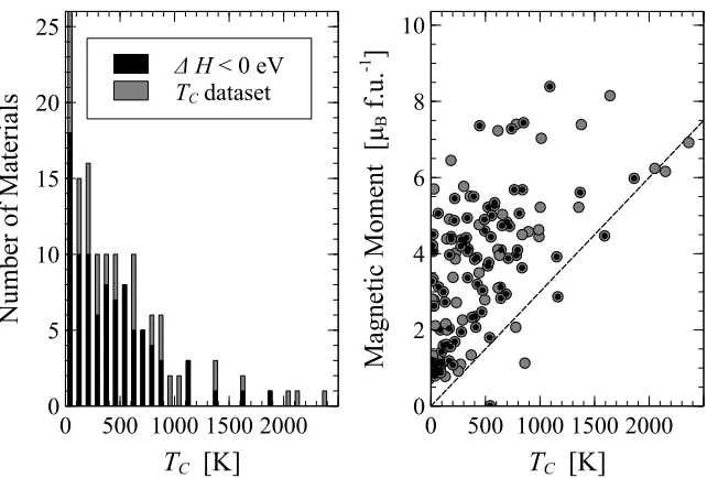
radius thus results in a strong overestimation of the TC. . . 73 2.5 The Curie temperature, TC, for the 229 material dataset, found by the

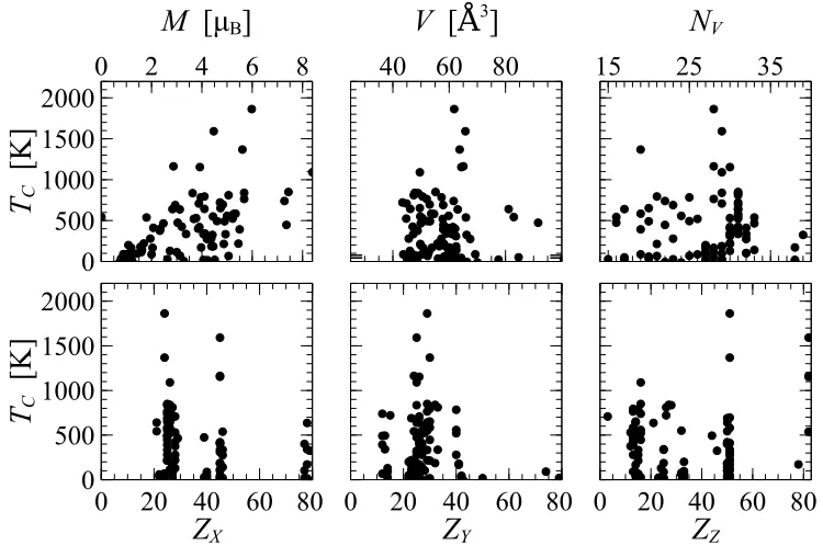
high-throughput screening procedure (cf. figure 2.1). Left Panel -the his-togram of TC for the whole dataset (grey) and the subset of potentially stable materials (black). Right Panel -the relationship between the mag-netic moment and theTC. A dashed line, having a slope of 0.003µBK−1, is shown to guide the eye. . . 74 2.6 The dependence of the Curie temperature, TC, on the structure and the

composition of the (X2Y Z) Heusler alloys. The data is shown only for the potentially stable alloys, ∆H <0 eV. TheTC is plotted as a function of the magnetic moment, M, the volume, V, the valence, NV, and the

2.7 Correlation of the magneto-crystalline anisotropy (MCA) with a number of structural and compositional parameters for the 229 material dataset (grey). The mutual dependence of all of the variables is shown. Namely, the MCA, the magnetic moment,M, the valence electron count, NV, the

volume, V, and the c/aratio. The compounds with a negative enthalpy of formation, ∆H < 0 eV are shown in black. . . 78 2.8 The dependence of the magneto-crystalline anisotropy (MCA) on the

va-lence of individual atoms,Ni, and the corresponding atomic numbers,Zi,

where i∈ {X, Y, Z}. . . 79 2.9 The magneto-crystalline anisotropy (MCA) as a function of the Curie

temperature, TC, and the magnetic moment. The MCA= 1 MJ m−3 and the TC = 500 K are indicated by the dashed lines. The stable materials, ∆H < 0 eV, which fall into this window make a viable candidates for permanent magnet applications. This is further discussed in the text. . . 80 2.10 Receiver operating curve (ROC) for the two hard magnet classifiers

dis-cussed in the text (left). The area under the curve (auc) is indicated in the brackets. The operating point of an ideal classifier, having auc= 1, is indicated by the arrow. In the right panel (bottom), a probability den-sity for the true positive, pi(x), and the true negative samples, n(x), is

shown, for two hypothetical classifiers. In the upper right panel we show the corresponding ROC curves. . . 83 2.11 Top panel -histogram of the site occupation for the 114 material training

set. The magnets have been labeled as “true soft”, “soft” and “mixed”. The first group is made from materials which have MCA ≤0.8 MJ m−3, as predicted by DFT. The second two groups are labeled according to the CLF2 prediction. The “soft” magnets are those, which are classified as positive, when the classifier operating point is set just before the knee in figure 2.10. In this case there is no misclassified samples. The negative samples are labelled as “mixed”, since they are a mixture of the hard and the soft magnets, that can not be resolved by the classifier. Bottom panel - a closer look at the trends in the mixed magnet group. Here the materials have been labeled as the “true hard” and the “true soft”, according to the MCA value predicted by the DFT. . . 86 2.12 The learning curve for the CLF2 classifier. . . 87

3.1 Illustrated density of states, D(E), of common magnetic metals. The absolute magnetic moment, M, and the spin polarization,P, are shown. The spin up and the spin down channel are denoted by arrows. a) para-magnet (M = 0 and P = 0), b) ferromagnet/ferrimagnet (M ≥ 0 and 0 %≤P ≤100 %), and c) half-metal (M ≥0 andP = 100 %) . . . 92 3.2 The SDFT ground state energy of Mn2Ga for three different magnetic

orders: the diamagnetic (diam), the ferromagnetic (ferrom), and the fer-rimagnetic (ferrim). The equilibrium lattice constants are indicated by the minima of the quadratic curves, obtained by fitting the energy as a function of the lattice constant. . . 97 3.3 Total energy and magnetization for Mn2Ga and Mn2RuGa, top and

3.4 Magnetism in cubic Mn2RuxGa compounds. a) Site projected magnetic moment for the two Mn sites, 4a and 4c, as a function of the lattice con-stant, a, and the Ru fraction, x. The vertical lines denote the Mn2Ga lattice constant as determined by the theory, 5.7 ˚A, and the experiment, 5.97 ˚A. b) Difference of the Mn magnetic moments, ∆M, as a function of the lattice constant (left) and the Ru concentration (right). The dashed line shows a linear interpolaton of the experimentally observed magneti-zation slope. . . 100 3.5 Electronic structure for stoichiometric Mn2RuxGa compounds at the

ex-perimental lattice constant, 5.97 ˚A. The unit cell is cubic. The spin up/down channels are shown in the upper/lower panel, respectively. . . . 101 3.6 Transport properties for three stoichiometric Mn2RuxGa compositions,

x = 0.33, 0.66 and 1.0. Fermi level position, Ef, is determined by the

va-lence electron number, NV. Left panel - Spin resolved resistivity (black)

and the corresponding DOS (blue). The data corespondingto the spin down channel is represented with negative values. Right panel - Calcu-lated transport spin polarization. . . 103 3.7 Isovolumetric energy profiles for stoichiometric Mn2Ga calculated at the

observed experimental and the relaxed DFT primitive unit cell volume, VEXP ≈ 52.9 ˚A and VDFT ≈ 46.4 ˚A, respectively. The theoretically ex-pected c/a ratios are denoted by the vertical dashed lines. ∆E is the energy difference between the experimental and the relaxed DFT struc-ture. Ed is the energy gain due to the formation of Ga defects. The net energy gain by forming the defects and taking the experimental structure is denoted byEg. . . 106 3.8 Calculated pressure for cubic MRG compounds at experimental (in-plane)

lattice constant, a= 5.97 ˚A, as a function of electronic doping, nel. . . . 108

3.9 Magnetic moment of Mn2RuxGa compounds. The DFT values calculated for stoichiometric compounds are shown by the green line. Correction to the DFT magnetization due to the formation of Ga defects is shown by the black points. The corresponding estimate of the Mn/Ga ratio is shown in the inset. The dashed line, equivalent to doping of 2eper Ru, is shown to guide the eye. . . 111 3.10 The spin resolved resistivity, ρ(E), and the corresponding spin

polariza-tion, P(E), as a function of energy. A scaled DOS is shown as a shaded background. The position of the spin gap is marked the divergence of the resistivity in the majority spin channel. . . 112 3.11 Calculated Mn2RuxGa spin polarization, for different levels of electron

doping, nel. The strain induced polarization is shown by the thick black

line. The experimentally reported range of values is shown by a shaded background. . . 113

4.2 Supervised learning. The ML approach consists of 5 steps: a) defining the problem, b) selecting and pre-processing the data, c) building the ML model, d)testing the model, and, finally,e) applying the ML model to the problem of interest. . . 122 4.3 The learning curve for the volume regressor. The score is plotted as a

function of the training set size. For each case the training and the vali-dation score are shown. The feature space is spanned by a 9-dimensional input vector of Eq. 4.1. . . 132 4.4 Accuracy of the volume regressor. Left Panel: The ML estimate is plotted

against the reference DFT data. The points which belong to the training set (189 points) are shown smaller (green). The test data (82 points) are shown in red. The line of the exact agreement with the reference data is shown in blue. Right Panel: The frequency at which the regression error occurs, as a function of its relative value (∆V /VDFT). The distribution was estimated from the test data. . . 132 4.5 Accuracy of the magnetic moment regressor. Left Panel: The ML

es-timate is plotted against the reference DFT data. The line of the exact agreement data is shown in red. Right Panel: The frequency at which the regression error occurs, as a function of its relative value (∆M /MDFT). The distribution was estimated from the test data. . . 135 4.6 a) Magnetic moment of the Fe atom as a function of the

next-nearest-neighbour atomic number, Z3, for a Wigner-Seitz radius of 2.7a0. The c/a ratio of the parent Heusler alloy is color coded. A machine learning estimate is shown by a solid blue line. b) The same data as previously, only now the radius of the points is proportional to the calculated enthalpy of formation, ∆H [210]. Large circles correspond to more stable alloys. . 137 4.7 Left Panel: Magnetic moment of Fe for a wide range of nearest neighbours,

at a constant Wigner-Seitz volume of ≈ 12 ˚A3. The atomic number of the next nearest neighbour, Z3, is color coded. We can notice a linear increase of the magnetic moment in the transition metal series which does not depend on Z3. The corresponding machine learning trend is shown as a blue line. Right Panel: a data sample containing a wider range of main group elements. The data elucidates the origin of the oscillation in the machine learning trend throughout the main group series in the left panel, indicated by a shaded ellipse. . . 139 4.8 The integrated charge (blue) and the magnetization (green) of Fe in the

TM2FeZ clusters, as a function of the transition metal (TM) atomic num-ber, ZTM. a) the total charge and the magnetization. b) the orbital resolved charge and the magnetization. The t2g and the eg orbitals are shown as full and doted line, respectively. c)The orbital resolved charge for the spin up and the spin down channel represented with positive and negative values, respectively. . . 141 4.9 Projected density of states of Fe in TM2FeZ clusters, where the selected

2.1 Summary of minimal required properties of a permanent magnet, namely the saturation magnetization,Ms, the uniaxial magnetic anisotropy

con-stant,Ku, and the Curie temperature, TC. . . 63 2.2 Comparison of the mean-field Curie temperature, TC, calculated using

the KKR,T_CKKR, and the FLEUR code,T_CF LEU R, with the experimental, T_Cexp, and the previously reported theoretical values, T_Cref [26, 137]. The temperatures are expressed in units of K. The calculation details are described in [138]. All calcualtions were performed for the regular cubic Heusler structure. The respective lattice constants, a, are shown in the table. . . 68 2.3 A list of candidate materials for permanent magnet application found

using the high-throughput screening approach described in this work. . . 80

3.1 A comparison of the experimental lattice constants,a, and magnetic mo-ments, M, for the Mn2RuxGa compounds with the corresponding DFT values. The respective units are ˚A and µBf.u.−1. . . 98 3.2 Calculated enthalpies of formation, ∆H, for the most stable competing

Heusler phases of the 1221 structural and magnetic Mn-Ru-Ga cells in-vestigated. The configurations investigated are limited to the primitive 4-atom Heusler cell (3-atom for half-Heuslers). . . 105 3.3 The electron doping estimate obtained using equation (3.6). The in-plane

lattice constant, aexp = 5.97 ˚A, andc/a= 1.02 are taken as parameters. . 110

The prosperity of modern society is mainly based on the constant development of new

technologies, allowing us to solve everyday tasks and problems more efficiently. Such

a development is enabled by the discovery of new materials, which underpin the new

technologies. For example, the development of the spin-valve [1] and the magnetic

tunnel junction [2, 3] has revolutionized the computer storage technology by making

high-capacity magnetic storage cheap and affordable to a wider range of consumers.

Online storage services have consequently become widely used by both companies and

individuals, transforming the way people live and work. Many other material classes,

like room-temperature superconductors, photovoltaics, thermoelectrics, and catalysts,

to name a few, have game changing potential. The desired properties are sometimes

intrinsic to a particular material, and hence easier to discover, but many require a

suitable combination of materials and environment conditions to manifest itself and that

is where the combinatorial possibilities explode. In such situations, classical research

methods e.g. experimental work, requiring man-work, time, and other resources, become

a bottleneck because they are hard to scale-up. Modern society requires that the new

discoveries and technological advancements are continuously achieved, putting a lot of

pressure on the research community. In order to accelerate discoveries new research

methods need to be developed.

The technological developments brought a significant advancement to the computer

tech-nology and computational science. These technologies nowadays offer a scalable solution

for the combinatorial bottleneck that impedes a fast material development. An

expo-nential increase in the available computational power over a period of 40 years has made

computers affordable and accessible to a large community of researchers. The continuous

development of computers has also resulted in the appearance of a number of computer

codes, which are used to calculate a variety of material properties. Many of these codes

are freely and easily accessible to the research community, thus enabling researchers

to simulate complex materials and phenomena with very little overhead, associated to

planning and setting up the experiment. One of the key advantages of computational

research is that one and the same computer can run an unlimited number of codes and

thus support the work of many research groups. This makes the computational research

relatively cheap, as compared to experimental work, and the production capacity can

be easily scaled-up.

The high-throughput (HT) methods are nowadays actively developed by the research

community, as a way to accelerate the material discovery. The defining trait of the

method is the exploration of a large, possibly opened, space of parameters [4]. To

exemplify what is meant by an open parameter space, one can imagine a HT search

for new stable structures, where the set of structures to be explored is not assigned in

advance but determined automatically during the search, e.g. by means of a heuristic

algorithm. Unlike the HT method, a combinatorial search has a limited and predefined

parameter space. Although there is no strict and generally accepted definition of the HT

method, it is worthy to mention the definition given by Curtarolo et al. [5]. According

to the authors, the HT method can be defined as: ” ... the throughput of data that

is way too high to be produced or analysed by the researcher’s direct intervention, and

must therefore be performed automatically: HT implies an automatic flow from ideas to

results”. The HT infrastructure involves both hardware and software, which facilitate

the HT workflow. The computational HT workflow begins with a candidate material

selection, followed by a large scale calculations of predefined properties, and finishes with

data post-processing (see figure 1). The previously described loop can be repeated, if

necessary, in order to refine the search using newly obtained results. The HT workflow

is also discussed in reference [6].

STORAGE STRUCTURES

HTP

workflow

I

II

III

OUT

IN

CALCULATION

DATA ANALYSIS

Figure 1: Simplified schematic of the computational high-throughput (HT) work-flow. First a set of preselected structures is passed to the automatized calculation engine, namely material properties are calculated and post-processed for storage into the database. In the final step the data in the database is subjected to the analysis. The results of the analysis may be the final objective of the HT calculation or just a new selection of structures can be made and fed into the input of the HT cycle. The Roman numerals denote the three key steps of the HT search: I) virtual materials growth, II)

The HT method has been applied to a wide range of investigations, namely in the search

of the thermodynamic stability of binary and ternary compounds [7–9], photovoltaics

[10], water photo-splitting [11] and catalysis [12, 13], carbon capture and gas storage

[14–16], scintilators [17], piezoelectrics [18, 19], thermoelectrics [20] and many more.

The need to process and interpret the HT results has driven the introduction of

data-mining and the machine learning (ML) methods into the material science [4, 21]. The

amount of data that is produced in such studies is overwhelming and precludes the

traditional, case study, investigations. The large amount of data, however, allows one

to adopt a completely new approach to materials science. The data produced by the

HT search can be analysed using a range of ML methods, e.g. principal component

analysis, clustering techniques, artificial neural networks, genetic algorithms, regression

methods, decision trees, self-organizing maps, etc. [22, 23]. The main aim of such studies

is to establish a correlation, or ideally a statistical model, between the properties of the

material and its structure, composition, etc., namely to extract the knowledge about

the structure-property relationship (SPR). The latter can then be used to optimize the

material properties. For example, the Slater-Pauling rule [24, 25] establishes a linear

dependence between the valence number of electrons and the magnetic moment of a

magnetic alloy. In some cases, simple (linear) relations can be found even for the highly

non-trivial properties, like the Curie temperature [26]. In general, the SPR will be

complex and multidimensional, and it can not be easily identified nor comprehended

by the human. In order to fully appreciate the problem, we need to consider that

HT data samples the (approximate) solutions for a large number of complex quantum

mechanical systems. The researchers task then is to find an “effective model”, which

can condense and distil these observations into a useful knowledge about the materials.

The statistical and the machine learning methods offer us new ways to do this, namely

to identify patterns, to extract knowledge, and to build the models in a data-driven

fashion. These methods thus have the potential to change how science is being done.

However, we are now in the midst of an early adoption stage, where the full potential of

these new tools still needs to be discovered and their utility demonstrated.

In this Thesis we will apply the HT and the ML methodology to the problem of finding

and engineering new magnetic materials. Magnetism and the magnetic devices are

im-portant for both applied and theoretical materials science. The latter being related to

the inherent complexity associated with the accurate description, and the

understand-ing, of the properties of the magnetic systems. The practical importance of magnetic

systems can not be overemphasized. We can freely say that the magnetic devices

un-derpin modern society. Magnets can be found in all segments of everyday life, from

high-performance electric motors and generators, to sensors, to electronics devices and

Figure 2: Crystal structure of the (X2Y Z) full Heusler alloys, also known as the

L21phase. TheZ atom is typically a main group element, occupying the 4b site. The

Y atom occupies the 4a site and the two X atoms occupy the 4c and 4d site. In the half-Heusler structure, C1b, the 4d site remains unoccupied.

are a few thousands of materials, which are known to order magnetically, perhaps only

a dozen of them have found practical applications [27]. The variety of magnets used

today, in the sense of performance and characteristics, has been obtained by material

engineering, by optimizing the composition and the production process. The discovery

of new magnetic phases, especially those suitable for the permanent magnet

applica-tions, has been scarce [28]. Here we investigate the magnetism in Heusler alloys. The

Heusler alloys are a versatile class of intermetallic materials with more than 1500 known

members [29]. The range of properties exhibited by these materials: metals, half-metals,

semiconductors, topological insulators, and many more, is extraordinary. The fact that

these materials crystallize in only two, fcc based, structures (C1b and L21) makes them

extremely appealing for applications. The properties of these materials can be tuned by

changing the chemical composition and there is no mismatch of crystal structures. The

crystal structure of the Heusler alloys is shown in figure 2. Since the unit cell consists of

3 to 4 atoms the number of material combinations to be explored is huge. All this makes

it an ideal set of materials for a HT study. In addition to the great potential that these

alloys have to offer, there is a strong (practical) reason for this choice. Namely, two large

HT databases [30, 31], containing information about 200 000 to 300 000 Heusler alloys,

are readily available. In particular, we use the data found in [31] as a starting point for

all our investigations.

The Thesis is structured as follows. In Chapter 1 we give an overview of density

func-tional theory (DFT), in particular its extension to magnetic systems. DFT is used

The basics of the electronic structure theory are reviewed. Our goal is to demonstrate

how the DFT information is used to describe the properties of real materials. Special

attention is devoted to the origin of magnetism in solids. We then discuss the methods

for calculating the magneto-crystalline anisotropy and the Curie temperature, which

are later used to characterize magnetic materials. Finally we give a gentle overview of

the statistical learning theory and discuss the practical aspects of the ML approach,

viewed as a function fitting problem. In Chapter 2 we design and test a HT screening

procedure for finding new permanent magnets within the family of the regular Heusler

alloys. The results of the HT investigation are used to identify the optimal composition

of a hard permanent magnet. Finally, a list of candidate materials, which meet all of

the HT screening criteria, is compiled. In addition, a simple statistical analysis allows

us to estimate the likelihood of finding new high-performance magnets. We then utilize

the ML classification in order to enhance the efficiency of the HT screening procedure.

In Chapter 3 we use the high-throughput data to perform a stability analysis of the

competing phases in Mn-Ru-Ga thin films, which show a great promise for realising a

fully-compensated ferrimagnetic half-metal [32, 33]. This is a material, which holds a

great promise for the application in spintronics [34]. By combining DFT investigation

and the HT data we identify the defects in these materials and investigate their effect on

the intrinsic material properties. We then construct models, which capture all the key

properties of the nominal Mn2RuxGa films, thus bridging a gap between the theoretical

(DFT) description and the experimental results. In Chapter 4, we build ML models

capable of describing the magnetism of Fe in regular Heusler alloys. In comparison to

other relevant materials science topics, magnetism has received very little attention in

terms of the application of the ML techniques [35, 36]. Due to the novelty of the ML

ap-proach, we discuss in great detail the practical aspects of building a ML model. These

considerations are then followed, step-by-step, in the construction of ML models for

magnetism. We use these models to identify and understand the physical origin of the

magnetic moment trends, with respect to the local chemical environment of Fe. Based

on the acquired knowledge, the ideal prototype for an Fe-based (X2F eZ) Heusler alloy

is postulated. We thus address the SPR directly. Using the ML models developed here,

we are able to characterize the magnetization for all alloys belonging to this prototype.

The most promising material candidates for the technological applications are identified.

The entire study is purely data-driven. No auxiliary DFT calculations have been

per-formed. We thus demonstrate the potential that the ML techniques have to offer in the

analysis of vast amounts of materials data and pave the way for the future data-driven

Theoretical Background and

Methods

1.1

The Electronic Structure Theory

The importance of materials for the development of the human civilization can not be

overstated. Ever since ancient history mankind has been shaping materials to aid them in

overcoming their daily challenges. The development of science, Physics and Chemistry

in particular, has allowed us to understand what makes certain, naturally occurring,

materials special; how to classify them, and how to make completely new functional

materials. This knowledge makes one of the pillars of the modern society. Today we

understand that all these properties arise from the interaction between the atoms. More

precisely, electrons interact with the atomic nuclei and with other electrons to give rise

to a wide spectrum of material properties. These interactions are described in full by

the laws of quantum mechanics. Since we know what are the relevant interactions in

any material, we can always write down the system of equations whose solution would

allow us to calculate any imaginable property of that material. In other words, today we

know how to write down the Hamiltonian for an arbitrary material and how to obtain

the solution, i.e. the wavefunction. Within the framework of quantum mechanics the

wavefunction contains all the information about the system. However, obtaining an

exact solution often represents an intractable problem.

Electronic structure theory (EST) is concerned with two issues that arise naturally. The

first is the necessity to establish the mathematical formalism and methods, which can

be used to solve the aforementioned problem in practice. The second is to provide a

formal connection between the quantum mechanical solution and the material properties,

which are sometimes phenomenological in character. For example: “Why does a material

have a silver or yellow color, or why is it transparent ?!” Likewise, one would hope to

provide an explanation for all the rules and the phenomena observed in Chemistry. The

core of the problem, which precludes finding an exact solution, in most of the cases, is

the interaction between a large number of electrons. In the absence of the latter the

material physics problem would be a rather simple one, namely it would be reduced to

an electrostatic problem. At the same time we would loose the concept of chemical bond

and life as we know would not be possible. Therefore, the description of electron-electron

(e-e) interactions is crucial for understanding of the properties of matter, which in turn

affect many aspects of our daily life.

Unfortunately, the interaction between a large number of electrons makes it one of the

most difficult problems in the entire physics. The crux of the problem lies in the fact

that the electrons are fermions and thus need to obey the Pauli exclusion principle. This

makes the problem intractable for more then a dozen of electrons. Any many-electron

wavefunction can, in principle, be represented as a linear combination of Slater

determi-nants [37], which satisfy the Pauli principle by construction. However, for moderately

large systems such a direct approach will likely never be feasible, due to the factorial

scaling. In practice, exact numerical solutions can be found only for very small

sys-tems, containing tens of electrons. Luckily, relatively simple approximations, like the

independent-particle approach, can be used to obtain a reasonably good description of

the electronic structure for a wide range of materials. Here the electrons are considered

as independent particles moving under the influence of an effective one-body

poten-tial, which describes the combined interaction with all other electrons in the system

in some approximate way. This approach was first pioneered by Hartree [38, 39] and

later developed by Fock [40]. Nowadays it is known as the Hartree-Fock method and

it represents the simplest wavefunction-based approach for solving many-body

prob-lems. Density functional theory (DFT) is another example of such an approach, which

is nowadays widely used as a universal tool to describe realistic materials [41]. Although

DFT is in principle an exact method, within the Kohn-Sham scheme it is reduced to

an independent-particle theory, where the e-e interactions are treated in an

approxi-mate way via an effective “mean-field” potential. Nevertheless, it is simple and accurate

enough to be considered as the most important method in electronic structure theory

today. The approaches which go beyond the independent-particle description are known

as the many-body methods. Here we can distinguish two main approaches, namely

the wavefunction-based and the Green’s function-based methods. The former are often

employed in chemistry and hence are known as the quantum-chemical methods. The

approach relies on a systematic expansion of the true many-body wavefunction in terms

of Slater determinants [42, 43]. This expansion in principle leads to a converging and

in terms of the admixture of different electronic configurations, which is important for

gaining chemical intuition, e.g. about the nature of the chemical bonds. The principal

shortcoming is that these methods can only be applied to small systems. The

investiga-tion of extended systems, e.g. solids, is not practically feasible using such an approach.

Since the physics of solids was, and still is, an active area of research, alternative

ap-proaches mainly based on the Green’s function methods were developed. The Green’s

functions allow an elegant interpretation of the many-body processes in terms of the

motion of particles and their interactions. These processes can be visualized in terms

of the Feynman diagrams [44], which makes the approach appealing to physicists. The

perturbation approach can be efficiently represented in terms of the Green’s functions.

The many-body problem can then be solved using an iterative approach, where at each

iteration the description of the e-e interaction can be refined. However, an important

point is that the e-e interaction is often large enough to make the perturbation approach

invalid. Therefore, the many-body methods often do not work with electrons directly

but instead use Green’s functions to define the equation of motion for quasiparticles, i.e.

for long lived excitations, which appear under the influence of the external

perturba-tion. By assumption, these quasiparticles are interacting via a weak force, namely the

screened Coulomb interaction, which makes the perturbation approach possible. The

problem here is to obtain the reasonable initial ground state for which the perturbation

can be applied. Lower level methods, like DFT or Hartree-Fock, are commonly used for

this. The second issue is related to the truncation of the interaction potential. More

specifically, it is hard to define a priori which diagrams will yield a rapidly converging

perturbation series. This makes the details of the approach problem specific. An

im-portant point is that the effective screened potential depends on the definition of the

quasiparticle, and hence the equations of motion need to be solved self-consistently. The

computational effort needed for this procedure is often prohibitive. The non-triviality

of the mathematical formalism, which underpins this approach, together with the

afore-mentioned practical limitations, confine the use of these methods to a number of

special-ist areas, e.g. for studying optical excitations. DFT is at the present the only method

which provides practically useful results while requiring a modest computational effort.

In addition, DFT has a low entry barrier, i.e. it easy for the beginners to start using it.

These are probably the main reasons why DFT is used so often in the condensed matter

physics today, despite all its shortcomings.

1.1.1 The Many-Body Problem

The properties of an arbitrary material can be determined from the solution of the

ˆ H =−1

2

X

i

∇2_i +1 2

X

i,j

1

|ri−rj|

−X

i,l

Zl |ri−Rl|

+ ˆE_ext(0)+ ˆHI . (1.1)

Here the indexigoes over all the electrons andlover all the nuclei of the system. Hartree

units, ~ =e = 4π₀ = 1 were assumed, with ebeing the electron charge and 0 the free

space permittivity. The atomic number of atoml is denoted asZl. The first two terms

in Eq. (1.1) describe the electronic degrees of freedom, i.e. the kinetic energy and the e-e

interaction, respectively. ˆHI denotes the Hamiltonian for the positively charged nuclei,

or simply ions. This term becomes relevant only when the ion dynamics is studied, e.g.

in phonon calculations. If the atomic centres are not allowed to move this term becomes

just an additive constant, which redefines the zero energy. In this case it does not play

an important role for the electron dynamics. The third term describes the electron-ion

interaction.

The operator ˆE_ext(0) represents an arbitrary external potential, e.g. a magnetic or an

electric field. It is often convenient to treat the electron-ion interaction as a part of the

external potential, in which case we can define

ˆ

Eext= ˆEext(0)−

X

i,l

Zl |ri−Rl|

, (1.2)

and the Hamiltonian can be symbolically expressed as

ˆ

H= ˆT + ˆHee+ ˆEext+ ˆHI. (1.3)

We note that the original Hamiltonian given by equation (1.1) is non-relativistic. The

leading relativistic corrections, namely the spin-orbit coupling, the mass-velocity and

the Darwin term [45], are often added as single-particle terms, after the many-body

problem has been replaced by an effective independent-particle system. The stationary

Schr¨odinger equation, defined by the Hamiltonian (1.3), then becomes

ˆ

HΨ({ri};{Rl}) =E Ψ({ri};{Rl}) , (1.4)

whereE is the total energy of the system and Ψ({ri};{Rl}) is the wavefunction, which

contains all the information about the system. The latter depends explicitly on both

the electronic and the ionic degrees of freedom. In most of the situations of interest the

ions move slowly enough compared to the characteristic electron time-scale, ≈10 fs, or

do not move at all. The characteristic time-scale for the vibrations is of the order of

ps. Therefore, the electronic degrees of freedom are in many cases practically decoupled

product of two terms

Ψ({ri};{Rl}) =ψ({ri})·Φ({Rl}) , (1.5)

where each term now depends exclusively on either the electronic or the ionic degrees of

freedom. The Schr¨odinger equation then decomposes into two equations, coupled by the

electron-ion interaction. This is known as the Born-Oppenheimer approximation. The

electronic part is solved first for a fixed ionic configuration, and then the force on the

ions can be evaluated and the ion positions updated. Since the ions have a large mass,

the quantum-mechanical phenomena associated with the wave nature of matter does not

usually manifest itself for them. For this reason the ions are often described using

semi-classical equation of motion. This further simplifies the problem. The non-semi-classical part

involves the action of the electrons on the nuclei, i.e. the electronic wavefunction is used

to evaluate the force on the nuclei. With the exception of hydrogen, this approximation

works very well for the usual range of temperatures and pressures. Matter under extreme

conditions requires special attention, which is out of the scope of this thesis. We note

that the ionic positions in the Born-Oppenheimer approximation define an effective

energy surface for the electrons. If the ions are allowed to move, these surfaces can

intersect and the approximation will break down. In this case a small displacement of

the nuclei can cause a large change in the electronic wavefunction. Therefore, as long as

the potentially energy surfaces are well separated and the motion of the nuclei can be

considered adiabatic the Born-Oppenheimer approximation will remain valid.

The independent-electron approximation, where the motion of individual particles is

unaffected by the other ones, at least not explicitly, is of great practical importance.

The most simple approach, which would result in such an approximation would be to

neglect the e-e interaction term altogether. In this case the motion of every electron

would be affected only by the electric potential of the ions and the individual electrons

would move in a completely uncorrelated manner. However, this approximation is often

not realistic. A more common approach is to take the e-e interaction into account in

some approximate way, e.g. via an effective one-body potential. An example of such a

model is the nearly-free electron model (see Ch. 7 in Ref. [46]), which was successfully

used in the early days of solid state physics to study the properties of metals. Despite

its simplicity, the approach allowed the development of many concepts in electronic

structure theory, like the concept of bands, Brillouin zone, etc. The opposite limit is

given by tight-binding models. Here one starts from an atomic reference state and treats

the electron hopping between the different sites as short-ranged. Although the physical

picture in these models is grossly simplified, they elucidate why the notion of atoms is

still relevant in solids and, more importantly, represent a great pedagogical tool. When

description of the electronic structure [47]. In this sense, they are still used in the solid

state physics research.

The most important extension of the previously discussed independent-particle approach

is the Hartree-Fock method (HFM). The crux of the method is to take the full

interact-ing Hamiltonian and to approximate the many-body wavefunction with a sinteract-ingle Slater

determinant. In this way the Pauli principle is satisfied by construction. Since the

wavefunction is expressed in terms of the single-particle orbitals, the method is unable

to describe completely the e-e correlations. By including additional degrees of freedom

in the wavefunction it is possible to further lower the energy of the system [48]. The

correlation induced by Pauli principle is known as the Fermi correlation. However, it

acts only between particles of the same spin (cf. equation 1.10). The correlation between

the electrons of different spin, due to the Coulomb interaction, is not captured by the

HF approximation. This is known as the Coulomb correlation. In order to capture

the latter, approaches that go beyond the HF are needed. In quantum-chemistry these

are known as the post-Hartree-Fock methods, e.g. the Møller-Plesset perturbation

the-ory, the configuration interaction and the coupled-cluster methods [42, 43, 49]. Within

many-body perturbation theory particle correlations are captured by the quasi-particle

self-energy operator [50] (see also Ch. A4 in Ref. [51]), which plays the role of an effective,

non-local, single-particle potential.

In order to gain a clearer insight into the problem of correlation, it is instructive to

express the 2-particle density,n(x,x0), using the normalized pair distribution function, g(r,r0), which is defined as

g(x,x0) = n(x,x

0₎

n(x)n(x0₎ . (1.6)

The single-particle density,n(x), and the two-particle density,n(x,x0), are defined as n(x) =N

Z

dx2 dx3 . . . dxN |Ψ(x,x2,x3, . . . ,xN)|2,

n(x,x0) =N(N−1)

Z

dx3 dx4 . . . dxN |Ψ(x,x0,x3, . . . ,xN)|2 , (1.7)

and x stands for a collective coordinate of the position and the spin, (r, s). The

“in-tegral” over the spin is just a shorthand notation for a summation. Naturally, the

definition of the pair distribution function makes sense only if we have two or more

electrons in the system. The Pauli principle then implies that, in a N-particle system,

the electrons form a single wavefunction, which is given in the simplest case by a single

Slater determinant. At all times the motion of electrons need to be such that the

an-tisymmetry of the wavefunction is preserved under particle permutation. This implies

interaction, can not be simply written as the product of the two single-particle densities,

i.e. n(x,x0)=6 n(x)·n(x0). The latter can be interpreted as the conditional probability of finding one electron, having spin s0, atr0 if the other one, having spins, is found at

r. By writing this as a product of two probabilities would mean that the two events are statistically independent, i.e. uncorrelated. However, this is not true. For fermions the

probability to find two particles in the same state is exactly zero. Using the definition

(1.6) we can write the e-e interaction energy, Eee, as

Eee=

1 2

Z

dx dx0 n(x,x

0₎

|x−x0_| =

1 2

Z

dx dx0 n(x)n(x

0₎

|x−x0_|

n(x,x0) n(x)n(x0₎ =

= 1 2

Z

dx dx0 n(x)n(x

0₎

|x−x0| g(x,x

0_{) =}

= 1 2

Z

dx dx0 n(x)n(x

0₎

|x−x0_| +

1 2

Z

dxdx0 n(x)n(x

0₎

|x−x0_| g(x,x 0₎₋₁

=

= 1 2

Z

dx n(x)

Z

dx0 n(x

0₎

|x−x0|+

1 2

Z

dxn(x)

Z

dx0 n(x

0₎

|x−x0| g(x,x

0

)−1=

= 1 2

Z

dx n(x)VH[n(x)] +

1 2

Z

dxn(x)VXC[n(x)] =

=EH +EXC . (1.8)

The first term is the Hartree energy, which represents the classical electrostatic

in-teraction, and the second one is the exchange-correlation energy. Therefore, the e-e

interaction term can be formally rewritten as a sum of single-particle terms, where the

electrons interact only with the effective potential field, Vef f =VH +VXC. This is an

exact expression. Note that onlyVXC is non-local and depends on the electron

correla-tion, now given by the unknown functiong(x,x0), which itself implicitly depends on the electron density. The practical problem is then to find a reasonable approximation for

the VXC. DFT, which is discussed in the next section, tells us that this potential can,

in principle, be chosen such that the exact many-body density, n(x), is obtained as a solution. However, in practice, the potential is always approximated.

From equation (1.8) we can see that when there is no correlation,g(x,x0) = 1, the second term vanishes, and we are left only with the electrostatic interactions. It is also

impor-tant to notice that the Hartree energy is divergent, due to the self-interaction. However,

this divergence is exactly cancelled out by the contribution from the exchange-correlation

term. In other words, the Pauli principle ensures that the e-e interaction remains finite.

Any approximation to the exchange-correlation term will leave the divergences

unbal-anced and, consequently, give rise to a self-interaction error. The VXC term lends itself

hole as

∆n(x,x0) =n(x,x0)−n(x)n(x0) , (1.9) which reduces to the exchange hole, ∆nX(x,x0), within the HF theory

∆nX(x,x0) =−δss0

X

i

φs_i(r)φs_i(r0)

2

. (1.10)

Where φs_i(r) are the single-particle spin-orbitals, which minimize the HF energy. It can be shown that the exchange hole integrates to one missing electron per electron at

position r. In general the Coulomb hole is a sum of the exchange and the correlation hole, where the latter only appears in approximations that go beyond the HF approach.

The effect of the correlation hole is to redistribute the electron density (see Ch. 3 in

Ref. [52]). Therefore, VXC describes the interaction of an electron with the Coulomb

hole that surrounds it. The “hole” corresponds to a decreased probability of finding a

second electron at the same position where the first one is located. In other words, every

electron is screened by the collective motion of all other electrons. If one electron moves,

the whole electronic cloud around it has to move, in such a way that the Coulomb hole

always tends to be centred at the position of the electron. Therefore, the electron and the

Coulomb hole behave in many respects like a single object, i.e. like a quasi-particle. This

behaviour is a direct consequence of the Pauli principle and makes the crux of the

many-body problem. Namely, the motion of a single electron is fundamentally inseparable

from the motion of all the other electrons. As a result the long range electrostatic

interaction is screened and has a much shorter effective range. This is the reason why

the independent-electron picture works so well for metals, where the screening is strong.

1.1.2 The Density Functional Theory

The density functional theory (DFT) is one of the most popular methods for the

calcula-tion of the electronic structure today. The origin of the method can be traced back to the

seminal paper of Hohenberg and Kohn (1964) [53], which proved that the ground state

of an interacting many-body system is uniquely determined by the electronic density.

The theory was later extended for a number of cases, e.g. to finite temperatures [54],

to time-dependent problems [55], to spin polarized and relativistic systems [56–58], etc.

Quantum mechanics teaches us that the information about the state of a quantum

sys-tem is contained entirely in the N-body wavefunction, which is formally a function of

3N spatial coordinates. For the time being we will omit discussing the spin degrees of

freedom. The Hohenberg and Kohn (HK) theorem tells us that the same information

is contained in the electron density, which is a function of only three coordinates. Even

which uniquely defines the Hamiltonian, the many-body wavefunction, Ψ(rN), and the ground state electronic density, n0(r), namely

V(r)←→Ψ(rN)←→n0(r) . (1.11) The Hamiltonian is assumed to be of the form

ˆ H=−1

2

X

i

∇2_i +1 2

X

i,j

1

|ri−rj|

+

Z

dr n(r)V0(r), (1.12) which is completely general, aside from a particular form of the last term, involving the

external potential. From a practical point of view, a Hamiltonian of this form covers

most of the known many-body problems. In other words, the HK theorem establishes

that the wavefunction is a functional of the electron density, Ψ(rN)≡Ψ [n(r)], and the isomorphism between the potential and the wavefunction implies that the Hamiltonian

is also a functional of the density, ˆH(rN_)≡Hˆ_v

0[n(r)]. In effect, the energy of the system

is a functional of the ground-state density

Evo[n0(r)] =hΨ [n0(r)]|Hˆvo[n0(r)]|Ψ [n0(r)]i . (1.13)

By virtue of the Rayleigh-Ritz variational principle it can then be shown that the

en-ergy functional (1.13) is variational, namely that an arbitrary, V-representable, electron

density, n(r)6=n0(r), always satisfies the inequality

E0 =Evo[n0(r)]< Evo[n(r)] , (1.14)

wheren0 is the true ground state density andEvo is the energy functional defined by it.

Provided that the latter is known, the ground state can in principle be obtained by

per-forming an energy minimization over all permissible densities, as implied by Eq. (1.14).

Unfortunately the HK theorem does not provide any indication on how to construct such

a functional. Even more so, despite 50 years of theoretical efforts, the form of the exact

functional is still unknown today. In order to implement the energy minimization of

Eq. (1.14) one needs to ensure that the trial densities are V-representable, namely that

a 1-to-1 mapping with the potential, in the spirit of Eq. (1.11), can be established for

all of them. Initially the hope was that all electron densities are V-representable, since

they represent a solution of a physical problem. However, counter-examples disproving

this assumption have been found [41]. In other words, not all electron densities are

V-representable.

The V-representablity problem is circumvented by the two step minimization procedure,

of V-representable densities, the Levi-Lieb (LL) approach suggests that the minimization

is first performed over a set of all N-electron wavefunctions, |ΨNi, which have density,

n(r). In the second step the minimization is performed over the established set of N -representable densities.

E0 = inf

n {Ψinf→nhΨ

N_{|Tˆ+ ˆH}

ee+ ˆV|ΨNi}=

= inf

n {

inf Ψ→nhΨ

N_{|Tˆ+ ˆH} ee|ΨNi

+

Z

drn(r)V(r)}= = inf

n {FLL[n(r)] +

Z

drn(r)V(r)} , (1.15) whereFLL[n(r)] is the Levi-Lieb functional, which is universal, i.e. it is independent of

the external potential V. Here inf denotes the infimum, i.e. the greatest lower bound.

The energy functional above becomes minimal for the same density that minimizes

the HK functional, and only for that density, which makes it a valid extension of the

true energy functional beyond the ground state. It turns out that any smooth

non-negative function n(r), which is normalized to the total number of electrons, N, is N-representable. However, despite such exact theoretical results a practical formulation

of the energy functional has proved elusive.

1.1.2.1 The Kohn-Sham Approach

The success of DFT is mainly due to the ansatz made by Kohn and Sham (KS), which

asserted that a true many-body electron density can be obtained as a ground state of

an equivalent independent-particle system, where the effective potential has been chosen

appropriately. This system is now known as the KS system. It was latter proved that

the KS approach makes an exact scheme (see Ch. 4 in Ref. [41]), provided that the

energy functional that generates the effective single-particle potential is known exactly.

In fact, this problem is equivalent to the original difficulties with the DFT approach

and hence, an exact functional was never obtained. Nevertheless, practically useful

approximations based on the KS scheme have allowed calculating the electronic structure

for large many-body systems, with sufficient accuracy needed to calculate, e.g. the

magnetic moments, the electric current under bias in nano- and molecular-junctions and

even to perform ab initio molecular dynamics. The latter is crucial to obtain relaxed

structures, which are a prerequisite for studying the electronic structure of realistic

systems, e.g. in the presence of defects, adsorbates on surfaces, etc. In addition, DFT

often represents a starting point for the more sophisticated many-body methods, which

and Chemistry. For this reason the 1998 Nobel prize in Chemistry has been awarded to

W. Kohn (together with J. A. Pople) for his contribution to developing DFT.

The KS approach asserts that the ground-state density of a fully interacting,

many-body system, can be obtained as the ground-state density of an equivalent system of

non-interacting electrons, the KS system. The N-electron density is defined as

n(r) =

N

X

i=1

|φi(r)|2 , (1.16)

whereφi(r) are the KS single-particle states.

The total energy functional

E[n(r)] =T[n(r)] +Eee[n(r)] +

Z

drn(r)Vext(r) , (1.17)

where both the kinetic energy, T[n(r)], and the e-e interaction energy, Eee[n(r)],

func-tional are unknown, can be rewritten as

E[n(r)] =TS[{φi(r)}] +EH[n(r)] +EXC[n(r)] +

Z

drn(r)V(r) . (1.18) Here the KS kinetic energy functional is defined as

TS[{φi(r)}] =−

1 2

N

X

i=1

hφi|∇2|φii , (1.19)

and represents a sum of single-particle kinetic energies. The Hartree energy and the

associated potentialVH, are defined in the same way as in equation (1.8). The

exchange-correlation (XC) functional,EXC, is formally given by

EXC[n(r)] =T[n(r)]−TS[{φi(r)}] +Eee[n(r)]−EH[n(r)]. (1.20)

We can see that it includes the many-body corrections to the kinetic and the e-e

interac-tion energy. Therefore, all the many-body effects remain implicit in the XC funcinterac-tional.

The advantage of the KS scheme is that the KS kinetic energy functional is given

ex-plicitly, while useful approximations can be obtained for the XC. The Rayleigh-Ritz

principle then leads to a set of N single-particle equations of motion (EOM) for the KS

orbitals

−1

2∇ 2_φ

i(r) +VS[n(r)]φi(r) =iφi(r) , (1.21)

Initial guess

n

Calculate

V

Solve KS equations

Ф

, ε

Calculate

n

Converged Mix Densities

n

n

Output Energy, force, stress

SCF Loop

NO

YES

Figure 1.1: Flow chart of the self-consistent loop used to solve the system of Kohn-Sham (KS) equations (1.21).

The XC potential is given formally by the functional derivative ofEXC,

VXC[n(r)] =

δExc[n(r)]

δn(r) . (1.22)

Since the KS potential, VS, depends implicitly on the KS orbitals, the KS system of

equations (1.21) needs to be solved using a self-consistent procedure. This is known as

the self-consistent-field (SCF) loop. The scheme of the procedure is shown in figure 1.1.

The loop is starts by making a guess for the density,nin, usually from the superposition of

atomic densities. Then the KS potential can be constructed and the system of equations

(1.21) solved, to obtain a set of KS orbitals. The latter define the new electron density,

nout, via Eq. (1.16). The new and the old densities are then compared. The iteration

stops when they differ by less then a specified tolerance. In this case the self-consistency

is reached. If the difference is greater than that, the two densities are mixed using an

appropriate scheme and a new trial density is constructed [61]. A new iteration of the

SCF loop can then be started. As a corollary of the HK theorem, all observable

ground-state quantities can, in principle, be calculated from the converged density. In practice,

the KS eigenstates are used to calculate the quantities of interest.

1.1.2.2 The Kohn-Sham Approach for Magnetic Systems

The previously discussed DFT formulation is also valid for magnetic systems, since the

formulate the DFT problem for the magnetic case is to explicitly use the magnetization

as an additional variable. In general, this leaves us with 4 independent scalar fields that

need to be varied in order to minimize the energy functional,E[n,m]. The extension of

DFT to magnetic systems, namely spin-DFT (SDFT), was first provided by von Barth

and Hedin (1972) [56]. In this case the scalar potential is replaced by a 2×2 matrix,

wαβ(r), acting on a 2-component spinor wavefunction, Ψ, where α, β ∈ {↑,↓}, are the

spin labels. The spinor components are the KS spin-orbitals,φiα(r). The density matrix,

nαβ(r), can be defined [56, 62] in terms of the KS spin-orbitals as

nαβ(r) =

occ

X

i

φ∗_iβ(r)φiα(r) . (1.23)

Similarly, the total energy functional is given as

E[nαβ] =hΨ[nαβ] ˆT+ ˆHee|Ψ[nαβ]i+

X

αβ

Z

dr nαβ(r)wαβ(r) . (1.24)

The electron density,n(r), can be obtained as

n(r) =T r(nαβ(r)) , (1.25)

where the trace is taken over the spin indices and the magnetic moment density, m(r),

as

m(r) =−µB T r



 X

β

nαβ(r)σβγ



 . (1.26)

Here σβγ represents a vector of Pauli matrices and µB = ₂~_me_e ≡0.5 (a.u.).

More explicitly, the four components of the density are

mx(r) =−(n↑↓(r) +n↓↑(r))·µB

my(r) =−i(n↑↓(r)−n↓↑(r))·µB

mz(r) =−(n↑↑(r)−n↓↓(r))·µB

n(r) =n↑↑(r) +n↓↓(r). (1.27)

Therefore, the density matrix of Eq. (1.23) can be rewritten as

nαβ(r) =

1

2n(r)δαβ− 1 2µB