Sliding Mode Control of Coupled Tanks System: Theory and an Application

International Journal of Emerging Technology and Advanced Engineering

Website: www.ijetae.com (

ISSN 2250-2459,

ISO 9001:2008 Certified Journal,

Volume 3, Issue 8, August 2013)

650

Sliding Mode Control of Coupled Tanks System: Theory and an

Application

Mohd Tabrej Alam

, Piyush Charan

, Qamar Alam

, Shubhi Purwar

1_{Department of Electronics & Instrumentation Engineering, Integral University, Lucknow, India} 2

Department of Electronics & Communication Engineering, Integral University, Lucknow, India

3_{Department of Electrical Engineering, Integral University, Lucknow, India} 4_{Department of Electrical Engineering, MNNIT, Allahabad, India}

Abstract –This paper deals with the level control of coupled tanks system using sliding mode control. A standard sliding mode control technique is proposed for the system. To reduce the chattering problem associated with the standard sliding mode control technique integral sliding mode control (ISMC) technique is proposed. The proposed control techniques guarantee the asymptotic stability of the closed loop system. To illustrate the developed control techniques the performance of the system is verified by MATLAB software. The simulation results indicate that the proposed control techniques work well.

Index Terms- Standard Sliding mode control; Integral sliding mode control (ISMC); Level control; Coupled tanks System.

I. INTRODUCTION

During the last three decades, variable structure systems (VSS) and sliding mode control (SMC) have received significant interest and have become well established research areas with great potential for different applications. Variable structure systems with a sliding mode control technique were discussed in the Soviet literature [1], [2], and have been widely developed in recent years. Comprehensive surveys of variable structure control given in [3], [4]. The salient feature of sliding mode control (SMC) derives from the property of robustness to structured and unstructured uncertainties once the system enters the sliding mode. Note that the system robustness is not guaranteed until the sliding mode is reached. The main drawback of sliding mode control is ―chattering‖ which can excite undesirable high frequency dynamics. Different methods of chattering reduction have been reported. One approach which places a boundary layer around the switching surface such that the relay control is replaced by a saturation function [6].

Sliding mode control technique is a type of variable structure control where the dynamics of a nonlinear system is changed by switching discontinuously on time on a predetermined sliding surface with a high speed, nonlinear feedback [7].

Actually, the procedure of sliding mode controller design has two steps: the first step is to obtain a sliding surface for desired stable dynamics and the second step is about obtaining the control law that provides to reach this sliding surface. The system trajectories are sensitive to parameter variations and disturbances during the reaching mode whereas they are insensitive in the sliding mode [8].

The discontinuous nature of the control action in sliding mode control is claimed to result in outstanding robustness features for both system stabilization and output tracking problems. A good performance also includes insensitivity to parameter variations and rejection of disturbances. Variable structure systems has been applied in many control fields which include robot control [9], motor control [10, 11], flight control [12], and process control [13].

In this paper, we propose a standard SMC and integral SMC techniques for the coupled tanks system. Simulation results are presented to illustrate the effectiveness of the proposed control techniques.

The paper is organized as follows: In section II the dynamic model of the coupled tanks system is obtained. In section III a standard sliding mode control technique is proposed for the system. In section IV integral sliding mode control (ISMC) technique is proposed for the system. The results of simulation are presented in section V. Finally concluding remarks and references are given in section VI and VII.

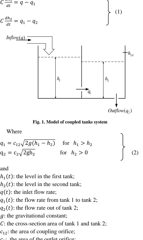
II. DYNAMIC MODEL OF COUPLED TANKS SYSTEM

International Journal of Emerging Technology and Advanced Engineering

Website: www.ijetae.com (

ISSN 2250-2459,

ISO 9001:2008 Certified Journal,

Volume 3, Issue 8, August 2013)

651

The dynamic model of the coupled tanks system can be written as-

(1)

2

( )

Outflow q

( )

Inflow q

1

h h₂

1 q

2d

h

Fig. 1. Model of coupled tanks system

Where

√ ( ) for

√ for (2)

and

( ) the level in the first tank;

( ) the level in the second tank;

( ) the inlet flow rate;

( ): the flow rate from tank 1 to tank 2;

( ) the flow rate out of tank 2;

the gravitational constant;

the cross-section area of tank 1 and tank 2;

the area of coupling orifice;

the area of the outlet orifice;

For the coupled tanks system, the fluid flow rate, into tank 1, cannot be negative because the pump can only pump water into the tank. Therefore, the constraint on the inflow rate is given by

(3)

now the governing dynamical equations of the coupled tanks system can be written as (Chang -1990)

̇ _{√ | | ( )}

̇ _{√ | | ( ) √ (4)}

at equilibrium, for constant water level set point, the derivatives must be zero, i.e.,

̇ ̇ (5)

thus, at equilibrium, the following algebraic equations must hold:

_{√ | | ( )}

(6)

_{√ | | ( ) √}

Where is the equilibrium inflow rate. From eqs. (6), and to satisfy the constraint in eq. (3) on the input flow rate, we should have ( ) , which implies

(7) therefore, in order to satisfy the constraint in eq. (3) on the input inflow rate for given values of plant parameter

and , the liquid levels in the tanks must satisfy the constraint in eq. (7). In addition, for the case when , the system model is decoupled. Thus, the general model suggested in [5] reduces to the model used in this paper which is the most widely used model in the literature when modeling the coupled tanks system.

Let

, , 0 1, ( )

and

√

, √

The output of the coupled tanks system is taken to be the level of the second tank. Therefore, the dynamic model in eqs. (1) and (2) can be written as

̇ √ √

̇ √ √ (8)

International Journal of Emerging Technology and Advanced Engineering

Website: www.ijetae.com (

ISSN 2250-2459,

ISO 9001:2008 Certified Journal,

Volume 3, Issue 8, August 2013)

652

The objective of the control scheme is to regulate the output ( ) ( ) ( ) to a desired value It is

easy to show using eqs. (8) that if ( ) ( ) is regulated to a desired value then ( ) ( )

( ) will be regulated to the value

The dynamic model of the coupled tanks system is highly nonlinear. Therefore, we will define a transformation so that the dynamic model given in eq. (8) can be transformed into a form facilitates the control design.

Let 0 1, and define the transformation ( )

such that

(9)

√ √

the inverse transformation ( ) is such

(10)

. √ /

It can be checked that we can write the dynamic model in eq. (8) as

̇

(11)

̇ .√

√ √

√ / √

Where the values of and in eq. (11) are function of and as given by eq. (10).

Hence, the dynamic model of the system can be written as

̇

̇ (12)

Where

.√

√ √

√ /

√

The dynamic model in eq. (12) will be used to design control techniques for the coupled tanks system.

III. STANDARD SLIDING MODE CONTROL

In this section, we will design a standard sliding mode controller for the coupled tanks system. Let be the desired output level of the system. i.e.,

The sliding surface ( ) is presented by Slotine and Li [14]

. / ̃

Where ̃ =tracking error and =order of

the system,

̇ ( )

_{√ √} ( ) (13)

on taking the derivative of eq. (13) w.r.t. time, we get

̇ .√

√ √

√ / √ ( √

_√ )

̇ ( √ √ ) (14)

on putting ̇ we get

, ( √ √ )-

since ( )

, ( _√ √ )- ( )

therefore standard sliding mode controller is

√ [ .

√ √

√

√ /

( √ √ ) ( )] (15)

Where and are strictly positive constant. And signum function is defined as

( ) {

International Journal of Emerging Technology and Advanced Engineering

Website: www.ijetae.com (

ISSN 2250-2459,

ISO 9001:2008 Certified Journal,

Volume 3, Issue 8, August 2013)

653

This asymptotically stabilizes the output of the system

( ) ( ) to its desired value

Stability analysis

Consider the Lyapunov function

(16)

on differentiating eq. (16) w.r.t. time, we get

̇ ̇ from eq. (14)

* ( _{√ √} )+

since, [ ̂ ( _{√ √} ) ( )]

where ̂ is estimation of . Therefore

̇ ,( ̂) ( )-

| | where | ̂|

if , then

̇ | | (17)

Where is a strictly positive constant, eq. (17) shows that the standard SMC technique guarantees the asymptotic stability of the closed loop system.

The proposed control technique suffers from the chattering problem. To reduce the chattering, integral sliding mode control (ISMC) is used, which is discussed in the next section.

IV. INTEGRAL SLIDING MODE CONTROL

In this section, we will design integral sliding mode controller for the coupled tanks system. Let be the

desired output level of the system. i.e.,

The sliding surface ( ) is presented by Slotine and Li [14]

( ) ∫ ̃ (18)

Where ̃ =tracking error and =order of the

system

̇ ( ) ∫ ( ) (19)

on taking the derivative of eq. (19) w.r.t. time,

̇ ( _{√ √} ) ( ) (20)

on putting ̇ we get

, ( √ √ ) ( )-

therefore integral sliding mode controller is

√ 0 .√

√ √

√ / ( √

_√ ) ( )1 ( ) (21)

where and are strictly positive constant.

This asymptotically stabilizes the output of the system

( ) ( ) to its desired value .

Stability analysis

Consider the Lyapunov function

(22)

̇ ̇ from eq. (20)

* ( _{√ √} ) ( )+

by using eq. (21), we get

̇ ,( ̂) ( )-

| | where | ̂|

if , then

̇ | | (23)

Where is a strictly positive constant, eq. (23) shows that the ISMC technique guarantees the asymptotic stability of the closed loop system.

V. SIMULATION RESULTS

Simulation of presented control techniques has been done using MATLAB software. Results are shown in Figures given below.

The dynamic model of the system has taken from [15], in which area of the orifices and

are given. The cross-section area of tank 1 and

tank 2 are found to be 208.2 . The gravitational constant is 981 . The desired value of the output of the system is taken to be = 5 .

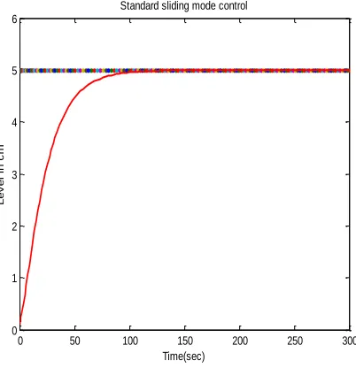
i. With standard sliding mode controller

The controller parameters used in the simulations are taken to be and . Figs. 2 and 3shows the simulation results when the standard sliding mode controller is used without input saturation. Fig. 2 shows that the output ( ) ( ) converges to its desired value

International Journal of Emerging Technology and Advanced Engineering

Website: www.ijetae.com (

ISSN 2250-2459,

ISO 9001:2008 Certified Journal,

Volume 3, Issue 8, August 2013)

654

Fig. 3 shows the control input in which chattering is evident and control effort is also very high. Fig. 4 shows that the output ( ) ( ) converges to its desired value

in about 115 s. Fig. 5 shows the control input, in which

control effort is greatly reduced.

The input constraint for the system is in the range:

.

1. Without input saturation

Fig.2. Liquid level in tank 2 by using SSMC

Fig.3. Liquid flow rate into Tank 1 by using SSMC

2.With input saturation

Fig.4. Liquid level in tank 2 by using SSMC

0 50 100 150 200 250 300

0 1 2 3 4 5 6

Standard sliding mode control

Time(sec)

L

e

v

e

l

in

c

m

0 50 100 150 200 250 300

20 30 40 50 60 70 80 90 100 110 120

Standard sliding mode control

Time(sec)

q

(t

)

in

c

m

3

/s

e

c

0 50 100 150 200 250 300

0 1 2 3 4 5 6

Standard sliding mode control

Time(sec)

L

e

v

e

l

in

c

International Journal of Emerging Technology and Advanced Engineering

Website: www.ijetae.com (

ISSN 2250-2459,

ISO 9001:2008 Certified Journal,

Volume 3, Issue 8, August 2013)

655

Fig.5. Liquid flow rate into Tank 1 by using SSMC

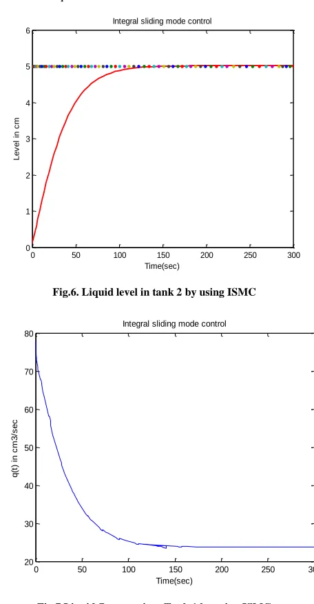
ii.With integral sliding mode controller

The controller parameters used in the simulations are taken to be and . Figs. 6 and 7shows the simulation results when integral sliding mode controller is used without input saturation. Fig. 6 shows that the output

( ) ( ) converges to its desired value in about

120 s. The control input shown in fig. 7; shows that the chattering as well as control effort is greatly reduced.Figs. 8 and 9 shows the simulation results when integral sliding mode controller is used with input saturation. Fig. 8 shows that the output ( ) ( ) converges to its desired value

in about 125 s. Fig. 9 shows the control input, in which

control effort and chattering are greatly reduced. The input constraint for the system is in the range:

.

1.Without input saturation

Fig.6. Liquid level in tank 2 by using ISMC

Fig.7 Liquid flow rate into Tank 1 by using ISMC

0 50 100 150 200 250 300

20 25 30 35 40 45 50 55

Standard sliding mode control

Time(sec)

q

(t

)

in

c

m

3

/s

e

c

0 50 100 150 200 250 300

0 1 2 3 4 5 6

Integral sliding mode control

Time(sec)

L

e

v

e

l

in

c

m

0 50 100 150 200 250 300

20 30 40 50 60 70 80

Time(sec)

q

(t

)

in

c

m

3

/s

e

c

International Journal of Emerging Technology and Advanced Engineering

Website: www.ijetae.com (

ISSN 2250-2459,

ISO 9001:2008 Certified Journal,

Volume 3, Issue 8, August 2013)

656

2. With input saturation

Fig.8. Liquid level in tank 2 by using ISMC

Fig.9. Liquid flow rate into Tank 1 by using I SMC

VI. CONCLUSION

Inthis study, the level control of coupled tanks system is proposed. The simulation result shows that integral sliding mode controller provides a better performance with respect to the standard SMC technique.

By using integral sliding mode controller, Fig.7 and 9 shows that chattering as well as control effort is greatly reduced as compare to standard sliding mode controller, and the control signal in Fig.9 is smoother than the control signal obtained from standard sliding mode control technique.

REFERENCES

[1] S. V. Emelyanov, Variable Structure Control Systems Moscow, U.S.S.R.: Nauka, 1967.

[2] V. I. Utkin, Sliding Modes and Their Application in Variable Structure Systems (in Russian). Moscow, U.S.S.R.: Nauka.

[3] R. A. DeCarlo, S. H. Zak, and G. P. Matthews,―Variable structure control of nonlinear multivariable systems: A tutorial,‖ Proc. IEEE, vol. 76, pp. 212–232, Mar. 1988.

[4] J. Y. Hung, W. B. Gao, and J. C. Hung, ―Variable structure control: A survey,‖ IEEE Trans. Ind. Electron., vol. 40, pp. 2–22, Feb. 1993. [5] Khan MK, Spurgeon SK, ―Robust MIMO water level control in

interconnected twin-tanks using second order sliding mode control,‖ Control Eng Pract 2006;14:375–86.

[6] J. J. Slotine and S. S. Sastry, ―Tracking control of nonlinear systems using sliding surfaces, with application to robot manipulators,‖ Int. J. Control, vol. 38, pp. 465–492, 1983.

[7] K.D. Young, V.I. Utkin, and U. Ozguner, ―A Control Engineer’s Guide to Sliding Mode Control,‖ IEEE Transactions on Control Systems Technology, vol. 7, no. 3, May 1999, pp.328-342. [8] J. Y. Hung, W. Gao, and J. C. Hung, ―Variable structure control: A

survey,‖ IEEE Transactions on Industrial Electronics, vol. 40, no.1, 1993, pp. 2-22.

[9] Sira-Ramirez H, Ahmad S, Zribi M, ―Dynamical feedback control of robotic manipulators with joint flexibility,‖ IEEE Trans Syst Man Cybernet 1992;22:736–47.

[10] Zribi M, Sira-Ramirez H, Ngai A, ―Static and dynamic sliding mode control schemes for a permanent magnet stepper motor,‖ Int J Control 2001;74:103–17.

[11] Alrifai MT, Zribi M, Sira-Ramirez H, ―Static and dynamic sliding mode control of variable reluctance motors,‖ Int J Control 2004;77:1171–88.

[12] Sira-Ramirez H, Zribi M, Ahmad S, ―Dynamical sliding mode control approach for vertical flight regulation in helicopters,‖ IEE Proc—Control Theory Appl 1994;141:19–24.

0 50 100 150 200 250 300

0 1 2 3 4 5 6

Integral sliding mode control

Time(sec)

L

e

v

e

l

in

c

m

0 50 100 150 200 250 300

20 25 30 35 40 45 50 55

Time(sec)

q

(t

)

in

c

m

3

/s

e

c