De Coupled Power System Analysis Using Parameter Injection Method

Full text

(1)Universal Journal of Electrical and Electronic Engineering 2(7): 286-293, 2014 DOI: 10.13189/ujeee.2014.020704. http://www.hrpub.org. De-Coupled Power System Analysis Using Parameter Injection Method Farhana Umer1,*, Syed Usman Sabir2, Noor Khan3, Muhammad Ali Mughal4, Hassan Gauhar5 Aftab Ahmed Almani5, Ghulam Fizza Shah6 1. Electrical Department, Mevlana University, Konya, Turkey Electrical Department, UCE&T, The IUB, Bahawalpur, Pakistan 3 Electrical Department, Mehran UET, Jamshoro, Pakistan 4 Electrical Department, Beijing University, Beijing, China 5 Electrical Department UCE&T, The IUBUCE&T, Bahawalpur, Pakistan 6 Telecommunication Department, The IUB, Bahawalpur, Pakistan *Corresponding Author: [email protected] 2. Copyright © 2014 Horizon Research Publishing All rights reserved.. Abstract In order to meet with the increasing demand of electrical energy and wide spread of energy consumers in an area, the decentralized power generation (DPG) is becoming more popular. In DPG mostly the renewable energy sources are used. These renewable energy sources acts as the small grids integrated into the main power system. Now for management, optimized operation and stability of the existing system the power flow analysis must be done at the connecting point of these grids. In order to perform load flow analysis the system analysis model is needed. In general system’s analysis, whenever the system structure changes we have to change the analysis model. As we know those DPG units are ‘in’ and ‘out’ of the system frequently, so this results in the change of the system structure. So every time the system structure is change we have to recreate the analysis model therefore by using the classical load flow analysis method, load flow calculation become complex. This paper introduces a new technique of parameter injection at the joining points of grid to reduce the load flow analysis complexity. There is no need to recreate the analysis model again and again whenever the system structure changes. Keywords Decentralized Power Generation, Renewable Energy Sources, Power Flow Analysis, Parameter Injection. 1. Introduction Electricity consumption is increasing day by day. It results in the expansion of energy market, so new energy sources which are mainly the renewable energy sources are rapidly integrating into the existing power system to meet the energy. demand. It gives rise to phenomena of decentralized energy generation. In decentralized energy generation bulk power is generated by incorporating many smaller units near to the load centre rather generating power at a centralized point, which is usually far away from the load centre. These decentralized units are mainly the renewable energy sources. “Figure 1”shows decentralized energy generation In “Figure 1”the renewable energy sources are integrating into the main power system. They share the power with the main power system through the connecting points. The decentralized energy units act as small grids [1, 2]. These units are Injecting power into the main power system. Whenever these grids are integrated into the power system the power flow between the connecting point of the grid and main power system should be known. This is necessary for the management, optimized operation, stability and the security of the power system, so each grid must have its own controlling units that monitors and control all these things [3, 4]. For controlling purpose we must know the power flow between the connecting point of the grids and the main power system. The “Figure.1” also shows different controlling units. In classical analysis of the power system bus admittance matrix plays an important role in defining the system structure or the analysis model. Whenever the new grid enters the existing matrix system the admittance matrix must be recreated as the system structure is changed. This results the complexity in the load flow calculation. So a new technique is needed to avoid this complexity due to the change in system structure. This paper proposed a technique of parameter injection at the joining point of the grids, so whenever system structure changes, we do not have to recreate the admittance matrix [5, 6]..

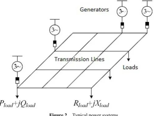
(2) Universal Journal of Electrical and Electronic Engineering 2(7): 286-293, 2014. 287. Figure 1. Decentralized energy generation.. 2. System Structure A typical power consists of different electrical elements such as generators, bus-bars, transmission lines etc. A typical power system is shown in a “Figure 2”. Figure 2. Typical power systems. We can use synchronous generator to represent a voltage source connected in series with impedance. In a power system different types of load are connected such as active load, reactive load, active current load, reactive current load, resistive load, reactance load and the apparent power load. The transmission lines that are used to connect the bus-bar can be represented by a pi-model or T-model. A power system shown in the “Figure 2” can be represented by the following “equation(1)”. 𝑌11 𝑉1 ⎡𝑉 ⎤ ⎡𝑌21 2 ⎢ ... ⎥ = ⎢ .... ⎢ ⎢ ... ⎥ ⎢ ... ⎣𝑉𝑛 ⎦ ⎣ 𝑌𝑛1. 𝑌12 … … . 𝑌22. … … . .. .. ... 𝑌𝑛2. 𝑌1𝑛 −1 𝐼1 ⎤ ⎡𝐼 ⎤ 𝑌2𝑛 .. ⎥ ⎢ 2... ⎥ .. ⎥ ⎢ .. ⎥ .. . ⎥ ⎢ .. ⎥ 𝑌𝑛𝑛 ⎦ ⎣𝐼𝑛 ⎦. (1). Where n is the number of buses in the power system 𝑉𝑖 =(𝑖 = 1,2,3,4, … . , 𝑛), is the complex vector of bus voltages. 𝐼𝑖 =(𝑖 = 1,2,3 … , 𝑛) is the complex vector of bus currents. 𝑌𝑖 =(𝑖 = 1,2,3 … , 𝑛) is the self admittance of bus i. The bus admittance plays key role in load flow calculation [7, 8]..

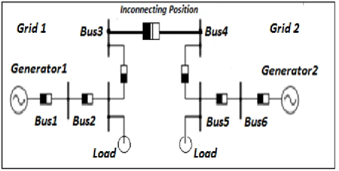
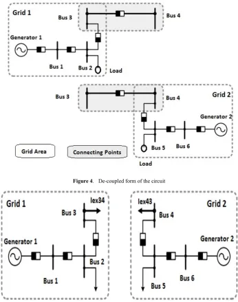
(3) 288. De-Coupled Power System Analysis Using Parameter Injection Method. Figure 3. connecting position of grids. 3. The Proposed Method As mentioned previously in classical method of power system we use bus admittance matrix and the bus admittance matrix depends upon system structure so we have to recreate the admittance matrix when the system structure is change due to the addition of new grid into the system. The new grids are frequently becoming ‘in’ and ‘out’ of the system due to the varying conditions resulting the frequent change in system structure. This made system analysis complex. That’s why a new technique of parameter injection is used to avoid complexity. This can be done by performing the following three steps: 1. 2. 3.. Locate the joining points of the grid Determine the exchanging parameter at the connection point Analysis on the individual area. 3.1. Locate the Joining Points of the Grids First of all we have to determine the connection points between the grid and the main power system as shown in the “Figure 3” The two grids are connected together the connection between two grids are third bus of the first grid and fourth bus of second gird 3.2. Determining the Exchanging Parameter at the Connection Point After the separation of two grids the structure is shown in “Figure 4”, it shows the exchanging parameters between the connection point that is the current and the voltage between connected buses. In order to calculate exchanging currents we have to use the hybrid calculations [5-7] in which the input parameters can be the applied current and the applied. voltage. To apply the hybrid method we first have to find the sorted bus admittance matrix by known parameters. The “equation (2)” shows the sorting of the bus admittance matrix where N is the index of the bus for which the bus current is known L is the index of the bus for the which the voltage is known than the hybrid matrix can be calculated as shown in “equation(3).. [𝐻] = �. [𝑌 ] [𝑌𝑁𝐿 ] � �𝑌𝑆𝑜𝑟𝑡𝑖𝑛𝑔 � = � 𝑁𝑁 [𝑌𝐿𝑁 ] [𝑌𝐿𝐿 ]. [𝑌𝑁𝑁 ]−1 [𝑌𝐿𝑁 Ι 𝑌𝑁𝑁 ]−1. −[𝑌𝑁𝑁 ]−1 [𝑌𝑁𝐿 ] � [𝑌𝐿𝐿 ] − [𝑌𝐿𝑁 Ι 𝑌𝑁𝑁 ]−1 [𝑌𝑁𝐿 ]. (2) (3). Now we use the hybrid matrix in our calculation to find the unknown voltages and currents. In the equation4𝑈𝑁 is known as voltage vector and 𝐼𝐿 is known as current vector. �. [𝑈𝑁 ] [𝐼 ] � = [𝐻] � 𝑁 � [𝐼𝐿 ] [𝑈𝐿 ]. (4). We can use iteration method to find the unknown buses voltages with the help of hybrid calculation as describe below  The first iteration process start from the first grid in order to find the terminal voltage of the third bus the input vector is the bus current vector from the first grid area and the voltage of the fourth bus, which is set to system nominal value.  The second iteration process is performed on the second grid area in order to find the terminal voltage of the fourth bus the input vector is the bus current vector from the second grid area and the voltage of the third bus which is calculated from the first iteration than the exchange current between the connected buses can be calculated by the voltage difference divided by the cable impedance[8-10].

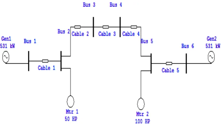
(4) Universal Journal of Electrical and Electronic Engineering 2(7): 286-293, 2014. 289. Figure 4. De-coupled form of the circuit. Figure 5. exchanging parameter between the grids. 3.3. Analysis of the Individual Area After the exchange parameter is calculated it will be added back to the corresponding bus. 𝐼𝑒𝑥 34 is added back to the third bus and 𝐼𝑒𝑥 43 is added back to the fourth bus the new structure is shown in the “Figure 5”. The exchange current represents the exchange power between the interconnected grids. Now analysis can be done on the individual area.. 4. Simulation In order to validate proposed analysis method the system shown in the Fig.6 is used We examine two cases in the simulation:. . . Firstly the system of two grids is considered as a single system and the system analysis results are obtained. Secondly the system is than separated or de-coupled into two individual grids. The exchanging parameter is injected at the separation points and the analysis results are obtained again.. To ensure the authenticity of the method analysis of results are compared. The parameters of the system are: two generators of same rating with rated apparent power 625 KVA, power factor is 0.8 the nominal voltage is 400𝑉𝐿−𝐿 , frequency is 60 HZ and two induction motors of 50 hp and 100 hp are acting as the load on each bus in the system connected with each other through a 100m cable having R=0.772 ohm/km and XL= 0.083 ohms/km..

(5) 290. De-Coupled Power System Analysis Using Parameter Injection Method. Figure 6. Simulation circuit. The output results of the generator are obtained from “Figure6”, which includes the current, active power reactive, power and power factor. 4.1. Complete System Analysis Result When the circuit is simulated the exchanging parameter between the two grids at the coupling point is obtained. It is 16 A current flowing from bus 3 to bus 4.. Figure 7. Analysis result of complete system. The current, active power reactive, power and power factor of generators are also obtained. These results are shown in Table 1..

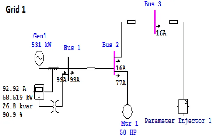
(6) Universal Journal of Electrical and Electronic Engineering 2(7): 286-293, 2014. 291. Table.1. complete power system analysis Complete Power System Analysis Result Parameters. Generator 1. Generator 2. Current. 92.92 A. 140.6 A. Active Power. 58.519 KW. 88.669 KW. Reactive Power. 26.8 KVAR. 40.3 KVAR. Power Factor. 90.9 %. 91.02 %. 4.2. Individual Grids Analysis Result After that the system is de-coupled into its constituents grids. Parameter injector is used at the de-coupling point to inject the same current as it was obtained during complete system analysis. Now both circuits are simulated saparately as shown in the “Figure 8”and” Figure 9”. Figure 8. Analysis result of Grid 1. Table.2. Grid 1 analysis result Grid 1 Analysis Result Parameters. Generator 1. Current. 92.92 A. Active Power. 58.519 KW. Reactive Power. 26.8 KVAR. Power Factor. 90.9 %.

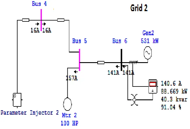
(7) 292. De-Coupled Power System Analysis Using Parameter Injection Method. Figure 9. Analysis result of Grid 2. Table.3. Grid 2 analysis result Grid 2 Analysis Result Parameters. Generator 2. Current. 140.6 A. Active Power. 88.669 KW. Reactive Power. 40.3 KVAR. Power Factor. 91.04 %. 4.3. Comparison of the Results Now the results obtained from both cases are compared in the table 4. It shows that the results from the two cases are exactly same only there is slight change in the power factor of generator 2 which is negligible. So in this way we can analyse any small grid parallel to main power system. Table.4 . Comparison of the Results Comparison Results Parameters. Generator 1. Generator 2. Complete System Analysis Result. Separate Grid Analysis Result. Complete System Analysis Result. Separate Grid Analysis Result. Current. 92.92 A. 92.92 A. 140.6 A. 140.6 A. Active Power. 58.519 KW. 58.519 KW. 88.669 KW. 88.669 KW. Reactive Power. 26.8 KVAR. 26.8 KVAR. 40.3 KVAR. 40.3 KVAR. Power Factor. 90.9 %. 90.9 %.

(8) Universal Journal of Electrical and Electronic Engineering 2(7): 286-293, 2014. 5. Conclusion The use of distributed energy generation is increasing now days to meet the energy demand. Distributed generation is obtained mainly from the renewable energy sources. They are acting like mini and micro grids integrating into the power system. It causes the frequent change in the power system structure. That results complexity in load flow calculation. In order to avoid this complexity the method of parameter injection at the integrating point is proposed, so whenever the system structure changes we do not have to recreate the analysis model. By using parameter injection technique the new grid integrating into the main power system can be analysed parallel to the main power system. In the simulation, system analysis is done by the proposed method. The comparison of results shows the accuracy of the method.. REFERENCES [1]. J. Farhangi,"The Path of the Smart Grid," IEEE Power & Energy, vol. 8, pp. 18-28, 2010; Jan/Feb.. [2]. Micro grids – Project, Project www.microgrids.eu/micro 2000. [3]. E. Ortjohann, P. Wirasanti, M. Lingemann, W. Sinsukthavorn,. website.. Available:. 293. S.Jaloudi, D. Morton, “Multi Level Hierarchical Control Strategy for Smart Grid Using Clustering Concept.”, ICCEP-International Conference on. CLEAN ELECTRICAL POWER Renewable Energy Resources Impact, Italy, 2011; June [4]. M. Lingemann, E. Ortjohann, W. Sinsukthavorn, S. Jaloudi, D. Morton,“Clustered Multi-level Hierarchy for Secondary Power System Control”, IASTED- Innovative Smart Grid Technologies for Sustainable Power and Energy Systems, Thailand,2010; November. [5]. K. Heuck, K.D. Dettmann, D. Schulz, Elektrische Energieversorgung, Vieweg, 2007, pp. 365-389.. [6]. A.J. Schwab, Elektroenergiesysteme, Springer Verlag, 2006, pp. 463-470.. [7]. J.J. Grainger, W.D. Stevenson Jr., Power System Analysis,4th ed. McGraw Hill Inc, 1994, pp. 238-280.. [8]. E. Ortjohann, O. Omari, Md. M. Rahman, D. Morton, “Active & Reactive Power Dispatch in Isolated mini-Grids Fed by Decentralized Power Sources”, 3rd International Conference on Electrical & Computer Engineering, 2004. [9]. E. Ortjohann, P. Wirasanti, W. Sinsukthavorn, S. Jaloudi, D. Morton “Analysis of interconnected power systems byhybrid calculation” international Conference on Renewable Energies and Power Quality (ICREPQ’11) Las Palmas de Gran Canaria (Spain), 2011; 13th to 15th April.. [10] P. Wirasanti, Student Member, IEEE, E. Ortjohann, S. Jaloudi, Student Member, IEEE, D. Morton “Decoupling power system analysis using hybrid load flow calculation.”.

(9)

No results found