Experimental Investigation and
Numerical Modelling of
Dynamic Behaviour of Screw Compressor Plant
Ekaterina Chukanova, Nikola Stosic
*, Ahmed Kovacevic
City University London, Northampton Square London EC1V 0HB, UK *Corresponding Author: [email protected]
Copyright © 2013 Horizon Research Publishing All rights reserved.
Abstract
An experimental and analytical study of screw compressor operation under unsteady conditions has been carried out. For this purpose a one dimensional model of the processes within a compressor was extended to include other plant components, including tanks and connecting piping. This was based on the differential equations of conservation of mass and energy. The results derived from the model have been verified by experiment in order to obtain a reliable tool that can simulate a variety of scenarios which may occur in everyday compressor plant operation. The analytical model was then further developed to demonstrate whole plant transient operation when a screw compressor is connected with storage tanks, control valves and heat exchangers in a complete system.Keywords
Screw Compressor, Compressor Plant, Dynamic Behaviour1. Introduction
Since most compressor plants rarely operate at steady conditions, an understanding of their behaviour during transient operation is vital. However, there are few publications that describe compressor operation under these conditions and most of those, related to positive displacement machines, refer to reciprocating compressors or complete compressor systems, as in refrigeration, air-conditioning, heat-pump, and process industry applications. Thus, for screw compressors, there is a need both for mathematical models, to predict their performance at unsteady conditions, and test data to validate these models. Start-up is one of the transient processes, which affect the performance and reliability of a screw compressor and the whole compressor system. There are several papers in the open literature which describe that process, generally addressing control problems and energy losses during transient operation. Jun and Yezheng [4], [5] carried out an experimental study of the effects of refrigerant migration during the start-up and shut-down cycles of a refrigeration system using a reciprocating compressor. They developed a
program for estimating energy losses due to this migration. Fleming, Tang and You [3] then published a paper on the simulation of shutdown processes in a screw compressor driven refrigeration plant. Their idea was to prevent reverse rotation by the use of a brake instead of a suction non-return valve. This, would decrease backflow significantly, through the clearances, and, consequently, reduce the shutdown torque. However, it has yet to be validated with experimental data. A disadvantage of reverse rotation braking is that it might cause failure if there is significant rotor backlash. Li and Alleyne [9] investigated start-up and shutdown transients in vapour compression cycle systems operating with semi-hermetic reciprocating compressors. They established a model of a moving boundary heat exchanger and validated it experimentally. Ndiaye and Bernier [11] developed a dynamic model of a reciprocating compressor during on-off cycle operation and validated it experimentally as part of a programme to justify water-to air heat pump models. A recent paper, by Link and Deschamps [10], describes both the numerical methodology and experimental validation of start-up and shutdown transients in reciprocating compressors.
splitting the machine into four subsystems, namely: the throttle-valve, the motor, the screw compressor block, and the oil/air separator, each described in a separate mathematical model. They emphasized that the warm-up and shut-down phases require a lot of energy and that this is often ignored when studying a compressor in the quasi-stationary state, thus, confirming the need for further study of screw compressor transients.
To reduce the number of experiments and to investigate cases which are difficult or not possible to measure, a mathematical model of a screw compressor plant under unsteady and dynamic conditions, based on the differential equations of continuity, momentum and energy was established.
2. Experimental Investigation
2.1. Test Rig Description
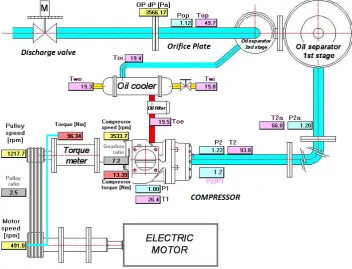
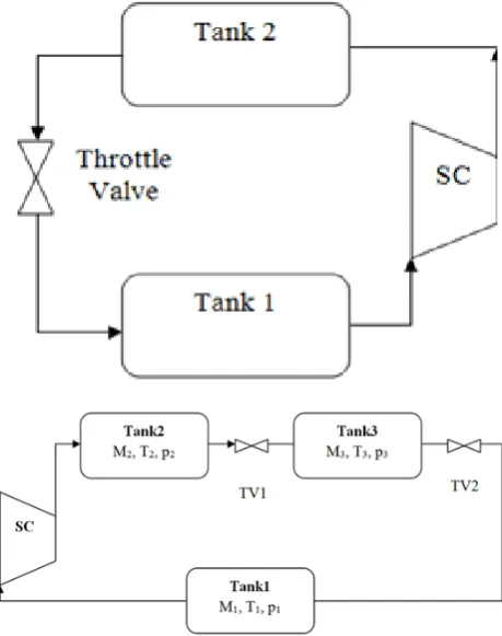
The experimental work was performed by utilization of an existing compressor test rig equipment, which is illustrated in Figure 1.
The oil-flooded twin screw compressor is driven by a six-band belt drive coupled to a 75 kW electric motor, the speed of which is controlled by a frequency inverter. A two stage oil separator, with a maximum working pressure of 15 bar, consists of two separator tanks which are joined together by a short pipe. The oil cooler is a shell and tube heat exchanger. This system does not have a pump since the oil is injected to the compressor by means of the pressure difference between the oil separator and compressor working
chamber. A motor driven throttle valve after the oil separator allows control of the air pressure inside the oil separator.
[image:2.595.322.542.166.331.2]The compressor that was tested, is shown in Figure 2. It has a 4/5 lobe configuration. The main rotor diameter d=128mm, while the length to diameter ratio (L/D) =1.2. The speed of the male rotor was kept constant, at 3000rpm, during the tests.
Figure 2. Tested compressor
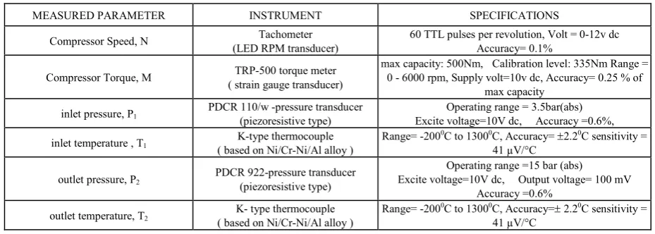
The measurements taken and the instruments used are described in Table 1, while the data acquisition system recorded measurements twice every second and saved the data in a separate file for further analysis. Before measurements were taken, the compressor was warmed-up for 30 minutes to make all temperatures along the casing uniform and to bring the oil temperature to the working level.
[image:2.595.130.483.465.734.2]Table 1. Test Rig Instruments
MEASURED PARAMETER INSTRUMENT SPECIFICATIONS
Compressor Speed, N (LED RPM transducer) Tachometer 60 TTL pulses per revolution, Volt = 0-12v dc Accuracy= 0.1%
Compressor Torque, M ( strain gauge transducer) TRP-500 torque meter max capacity: 500Nm, Calibration level: 335Nm Range = 0 - 6000 rpm, Supply volt=10v dc, Accuracy= 0.25 % of
max capacity
inlet pressure, P1 PDCR 110/w -pressure transducer (piezoresistive type) Excite voltage=10V dc, Accuracy =0.6%, Operating range = 3.5bar(abs)
inlet temperature , T1 ( based on Ni/Cr-Ni/Al alloy ) K-type thermocouple Range= -200
0C to 13000C, Accuracy= ±2.20C sensitivity =
41 µV/°C
outlet pressure, P2 PDCR 922-pressure transducer (piezoresistive type)
Operating range =15 bar (abs) Excite voltage=10V dc, Output voltage= 100 mV
Accuracy =0.6%
outlet temperature, T2 ( based on Ni/Cr-Ni/Al alloy ) K- type thermocouple Range= -200
0C to 13000C, Accuracy=± 2.20C sensitivity =
41 µV/°C
Several types of compressor starts were investigated, namely: starting from atmospheric pressure at the compressor discharge, starting from higher discharge pressures, starting with the discharge port open, and starting with the suction valve open and closed. All the recorded data were analysed to determine any trends and patterns in the screw compressor working parameters.
2.2. Presentation of Test Results
The aim was to observe the behaviour of the compressor before oil injection started. It was expected that, during that time, the temperature would rise quickly and might cause either loss of performance or damage.
As shown in Figure 3, when the compressor started from atmospheric pressure, the temperature increased from 55o to
100oC and then decreased after 8 seconds due to oil-injection,
since some time was needed for the pressure to build up in the oil reservoir sufficiently to admit the oil into the machine.
Figure 3. Start from atmospheric pressure at discharge
The situation is different when the compressor started with discharge pressures higher than atmospheric pressure, as
[image:3.595.316.547.412.614.2]shown in Figure 4. In this case, when the compressor stopped, oil flowed into the compressor due to the pressure difference, but the compressor filled with oil because the rotors did not rotate. So, when rotation began, the oil flowed immediately into the compressor and the temperature dropped until it stabilized soon after. In the first case, shown in Figure 3 when the compressor stopped, the discharge was open and all the oil flowed out of the compressor. As a consequence, when the compressor started, the compressor was empty, there was no oil inside and there was no pressure difference to make the oil flow.
Figure 4. Start at increased discharge pressure
This was a period of dry contact between the rotors, which could be decreased by closing both, the compressor suction and discharge ports during start up. When the compressor started, the pressure difference increased immediately, due to the suction pressure drop, as shown in Figure 5.
As a result there was a significant temperature rise from 50o to 90oC during the first 2 seconds, due to the high
[image:3.595.60.296.508.710.2]Figure 5. Start with closed suction
The un-lubricated period was decreased from 8 seconds for an ordinary start, to only 2 seconds for the start with the suction valve closed, as shown in Figure 3. After 32 seconds, the suction valve was open manually and the temperature rose again, as shown in Figure 5. This does not imply that there was no oil inside but because there was increased suction inflow with insufficient oil to maintain the temperature at the same level.
The temperature increased in the following 2 seconds until the pressure difference built-up and more oil was injected but the second increase was less significant than the first, with an increase from 55o up to 70oC during this phase.
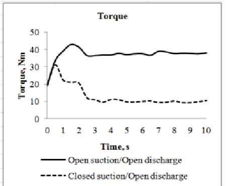
[image:4.595.66.290.79.279.2]There are other benefits from starting the compressor with the closed suction, as can be seen by comparison between Figure 3, showing an ordinary start, with Figure 6, which shows starts with open and closed suction. As soon as the suction is closed, the compressor is started, the suction pressure approaches vacuum conditions and air flow is almost zero. At the same time, the discharge pressure is equal to the atmospheric pressure (Figure 6, bottom) as is the case when the discharge is open.
Figure 6. Comparison of start with open and closed suction Due to the small pressure difference and low air flow, the peak torque (Figure 6, top) was approximately one third less than during start with open suction and the starting torque was about four times less. As a consequence, start up is safer with lower power consumption and less noise.
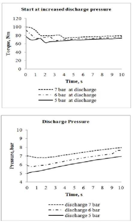
[image:4.595.324.545.357.735.2] [image:4.595.68.295.548.733.2]After starting the compressor under varying conditions, it was found out that the higher discharge pressure, the more time was required for the compressor to achieve 3000 rpm (Figure 7, top) and its acceleration was lower (Figure 7, bottom). It can be seen clearly that the slowest start up time and the lowest acceleration was at 7 bar at discharge pressure, with the times for 6 bar and 5 bar progressively shorter. Attempts were made to start the compressor with 8 bar at its discharge, but, since the motor current was limited, the compressor failed to start for all discharge pressure higher than 7 bar.
Consequently, as shown in Figure 8, the starting torque was highest at 7 bar and lowest when it started at 5 bar. It should be noted that when the compressor started with 5 bar
discharge pressure, the discharge pressure start ed to increase immediately, but at 6 and 7 bar, the discharge
[image:5.595.68.290.285.655.2]pressure first decreased before starting to rise.
Figure 8. Torque and discharge pressure curves for starts with different discharge pressures
3. Analytical Studies
The model developed is for numerical simulation of unsteady behaviour of a screw compressor within a
compressor plant, including the filling and emptying of the plant tank and associated connecting pipes during different types of compressor starts. The plant model has been integrated with SCORPATH (Screw Compressor Optimal Rotor Profiling and Thermodynamics), an existing compressor design program, developed in house.
The model is written in FORTRAN and is based on the differential equations of mass and energy conservation, developed and tested in earlier work. It is sufficiently general to take into account dry and oil flooded compressors and various plant tanks connected by gas pipes in different combinations providing that they are characterized by one volume and one exit valve.
3.1. Mathematical Model of the Screw Compressor
The screw compressor model is based on the simultaneous analysis of the thermodynamic and fluid flow processes, both of which are dependent on the screw compressor geometry. This is defined by a set of equations which describe the physics of the complete compression process.
The equation set consists of the equations for the conservation of energy and mass continuity together with a number of algebraic equations defining the flow phenomena in the fluid suction, compression and discharge processes combined with a differential kinematic relationship which describes the instantaneous operating volume and its change with rotation angle or time. In addition, the model accounts for a number of 'real-life' effects which may influence the final performance of a real compressor and make the model valid for a wider range of applications.
In the past, these equations have often been simplified in order to achieve a more efficient and economical numerical solution of the set. In this case, where all the terms are included, the effect of such simplifications on the solution accuracy can be assessed.
The working chamber of a screw machine together with the suction and discharge plenums can be described as an open thermodynamic system in which the mass flow varies with time and for which the differential equations of conservation laws for energy and mass are derived using Reynolds Transport Theorem.
A feature of the model is the use of the unsteady flow energy equation to compute the effect of profile modifications on the thermodynamic and flow processes in a screw machine in terms of rotational angle, or time.
The following conservation equations have been employed in the model.
The conservation of internal energy and mass is presented in equations (1):
(1)
in out
dm m m d
ω
θ
= − in in out out
dU
m h m h
Q
p
dV
d
d
ω
ω
θ
θ
=
−
+ −
where θ is angle of rotation of the main rotor, h=h(θ) is specific enthalpy, m m =
( )
θ is the mass flow rate, p=p(θ) is the fluid pressure in the working chamber control volume, Q=Q(θ) is the heat transfer between the fluid and the compressor surrounding and V=V(θ) is the local volume of the compressor working chamber.Flow through the suction and discharge ports is calculated from the continuity equation. The suction and discharge port fluid velocities are obtained through the isentropic flow equation. The computer code also accounts for reverse flow.
Leakage in a screw machine is a substantial part of the total flow rate and affects the compressor delivery, i.e. volumetric efficiency and the adiabatic efficiency, the gain and loss leakages are considered separately. The gain leakages come from the discharge plenum and from the neighbouring working chamber with a higher pressure. The loss leakages leave the chamber towards the discharge plenum and to the neighbouring chamber with a lower pressure. The leakage velocity through the clearances is considered to be adiabatic Fanno-flow through an idealized clearance gap of rectangular shape and the mass flow of leaking fluid is derived from the continuity equation. The effect of fluid-wall friction is accounted for by the momentum equation with friction and drag coefficients expressed in terms of Reynolds and Mach numbers for each type of clearance.
In addition to lubrication, the main purpose for injecting oil into a compressor is to cool the gas. The solution of the droplet energy equation in parallel with the momentum equation yields the amount of heat exchange with the surrounding gas.
The injection of oil or other liquids, for lubrication, cooling or sealing purposes, modifies the thermodynamic process substantially. The same procedure can be used to estimate the effects of injecting any liquid but the effects of gas or its condensate mixing and dissolving in the injected fluid or vice versa should be accounted for separately.
The equations of energy and continuity are solved to obtain U(θ) and m(θ). Together with V(θ), the specific internal energy and specific volume u=U/m and v=V/m are now known. T and p, or x can then be calculated. All the remaining thermodynamic and fluid properties within the machine cycle are derived from the pressure, temperature and volume directly. Computation is repeated until the solution converges.
For an ideal gas, the internal thermal energy of the gas-oil mixture is given by (2):
( )
( )
(
)
1
gas oil oil
mRT
U
=
mu
+
mu
=
γ
+
mcT
−
(2)(
1
)
U
(
mcT
)
oilT
mR
γ
−
=
−
Hence, the pressure or temperature of the fluid in the compressor working chamber can be explicitly calculated by the equation for the oil temperature Toil.
For the case of a real gas the situation is more complex, because the temperature and pressure can not be calculated explicitly. However, since the equation of state p=f1(T,V)
and the equation for specific internal energy u=f2(T,V) are
decoupled, the temperature can be calculated numerically from the known specific internal energy and the specific volume obtained from the solution of the differential equations, whereas the pressure can be calculated explicitly from the temperature and the specific volume by means of the equation of state.
In the case of a phase change for a wet vapour during the compression process, the specific internal energy and volume of the liquid-gas mixture are (3):
(
1
)
f g(
1
)
f gu
= −
x u
+
xu
v
= −
x v
+
xv
(3) where uf, ug, vf and vg are the specific internal energy andvolume of liquid and gas and are functions of saturation temperature only. The equations require an implicit numerical procedure which is usually incorporated in property packages. As a result, temperature T and dryness fraction x are obtained. These equations are in the same form for any kind of fluid, and they are essentially simpler than any others in derived form. In addition, the inclusion of any additional phenomena into the differential equations of internal energy and continuity is straightforward. A full account of the compressor model used in this work can be found in Stosic, Smith and Kovacevic [15].
3.2. The Unsteady Process in a Lumped Volume of the Plant Reservoirs and Connecting Pipes
An interface was written to couple the compressor and plant model elements for this purpose and has been used to show how the tank pressure is affected by the gas mass flow rate, the compressor discharge gas temperature, and the volume of the tank and communicating pipes.
A two tank plant model was investigated which enables closed systems to be simulated, such as refrigeration, air-conditioning and heat pump plants, as well as plants which operate under power cycles, like those of Joule and Rankine. In fact, since a one tank model is a special case of this and if the volume of the compressor inlet tank is assumed to be very large or infinite, this may be used to simulate the atmosphere. Thus, a developed two tank model can be used to obtain one tank model results.
Both two and three tank plant are illustrated in Figure 9. In the two tank case, gas from Tank 1 goes to the compressor suction and is then, discharged to Tank 2 and returns to Tank 1through a throttle valve.
for that analysis in finite difference form are as follows (4): (4) where indices 1 and 2 denote the start and end time of filling/emptying respectively and ∆t is the time difference between them.
Figure 9. Two and Three Tanks schematics
If the compressed gas is assumed to be the ideal, the finite difference equations can be written as (5):
2 1
R t
(
in in out out)
p
p
m T m T
V
γ ∆
=
+
−
2
2 2
2
2
m
V
p
T
R
ρ
ρ
=
=
2 2 0
2 (
)
out
m
=
µ
A
ρ
p p
−
(5) To estimate the unsteady behaviour of a compressor plant system, the tank equations are coupled with the compressormodel equations and solved in sequence to obtain a series of results for each time step. When the pressure p2 in the tank at
each time step is known, the flow and temperature min and
Tin at the compressor discharge can be calculated. These
derived valuesare then taken as the input parameters for the next time step. When the tank pressure p2 is calculated, mout
is either known, or calculated as the flow through the exit throttle valve to pressure p0 and T2 becomes Tout in the next
time step. The calculation is repeated until the final time is reached.
Mass inflow and outflow were calculated as pipe flows with restrictions which comprised the line and local losses, thus defining pressure drops within the plant connections. Since the tanks are of far higher volume than the connections, the gas velocities within them are much lower, and the pressurse losses in the tanks are significantly lower than those in the pipe.
Two levels of programming were applied. First, the compressor and plant processes were solved separately. The compressor process was then calculated through proprietary software and the tank model was processed, by mutual interchange of output and input data. Since this combination appeared to be slow in data transfer, the compressor and tank procedures were programmed together, to get instant data exchange. This resulted in very rapid calculation, allowing the bulk estimation of unsteady behaviour of screw compressor plant in a variety of scenarios.
3.3. Experimental Verification of the Results Obtained from the Mathematical Model
The model was verified by comparison of predictions obtained from it with measurement results obtained in a series of tests performed on the compressor test rig. More details of the tests are given by Chukanova, Stosic and Kovacevic [1,2].
The compressor, described in Section 3, was used to test the plant model viability for several operating conditions. The results are presented in groups on the basis of variation of the throttle valve area, variation of the tank volume and tank pressure, as well as variation of the compressor shaft speed. Both two tank and multi tank plant models were considered.
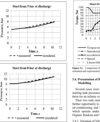
The experimental and predicted results of pressure variation during the start up, presented in Figure 10 for the starting receiver pressures 5 and 8 bars, show good agreement.
(
)
(
)
2 2 1 1
2 1
in in out out in out
m u
m u
m h
m h
t
m m
m
m
t
−
=
−
∆
−
=
−
∆
Figure 10. Comparison of pressure variation in the tank during the compressor start up at 5 and 8 bars
The most illustrative diagram in the comparison of experimental and predicted results is presented in Figure 11. It represents torque, shaft speed and shaft acceleration, which latter feature is the most critical criterion for comparison, since it indicates what parts of the starting curve correspond to friction and inertial effects.
Figure 11. Comparison of torque, shaft speed and acceleration between simulated and experimental results
3.4. Presentation of Results Obtained by Mathematical Modelling
Several cases were presented and analysed for variety of starting tank pressures, tank volumes and valve areas, all of them for an infinite volume inlet tank or atmosphere.
Then two tank model results were presented which give further opportunity to test closed systems, like refrigeration, air-conditioning and heat pump plants, as well as plants which operate under power cycles, like Joule, Rankine, Organic Rankine and Wet Rankine cycles.
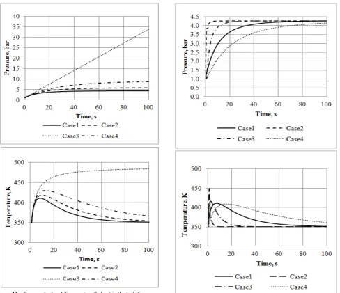
3.4.1. Variation of Valve Area
The throttle valve area was varied for the following cases. Case 1 – Av=70mm2, Case 2 – Av=50 mm2, Case 3 –
closed valve, Case 4 – Av=30 mm2
From the curves shown in Figure 12, it can be seen how the pressure and temperature change for different valve areas. For example for the case of the closed valve between the tanks, the pressure in the tank reaching 33 bar in less than 2 minutes and the temperature of the air increasing from 350K (77°C) to 450K (177°C) in just 10 seconds. In fact, this confirms how the valve area can be used to control the discharge pressure.
-50 0 50 100 150 200 250 300
0 10 20 30 40 50 60 70 80 90 100
0 1 2 3 4 5 6 7 8 9 10
To
rque
, N
m
Time, s
Start from 7 bar at discharge
Torque measured
Simulated Torque with mech losses acceleration
Speed
Linear (Simulated Torque with mech losses)
Spe
ed,
1
/s,
A
cce
le
ra
tio
n,
1
[image:8.595.76.401.84.480.2]Figure 12. Pressure (up) and Temperature (below) in the tank for cases with different valve areas
3.4.2. Variation of Tank Volume
The tank volume was varied as follows: Case 1 – V=0.3m3,
Case 2 – 0.03m3, Case 3 – 0.1m3, Case 4 – 0.6m3.
It can be seen from the curves in Figure 13 that for a given throttle valve area, the final discharge pressure will be the same for different tank volumes. It is only a question of the time for it to reach its final value: for a tank of 30 litres it will be 2 seconds, for 600 litres about 2 minutes. Similar characteristics apply to the temperature: the less volume the faster temperature reaches its peak (400-420K) and the faster that it returns to its initial value of 350K.
Figure 13. Pressure (up) and Temperature (below) in the tank for cases with different tank volumes
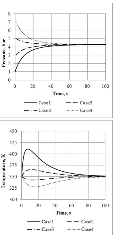
3.4.3. Variation of Tank Pressure
[image:9.595.64.553.81.502.2]Figure 14. Pressure (left) and Temperature (right) in the tank for cases with different starting pressure in the tank
3.4.4. Two Tank Case
This case, with a fixed valve area is presented in Figure 15 after the pressure in the inlet and discharge tanks stabilised for 4500 rpm. Further increases in shaft speed increased, the pressure in the discharge tank, while the pressure in the inlet tank decreased.
[image:10.595.312.549.76.272.2]Figure 16 shows the effect of a sudden change in the compressor shaft speed during the plant operation. The pressure in the discharge tank is doubled when the shaft speed is doubled. In this case, the volume of the inlet tank is kept much larger than that of the discharge tank.
Figure 15. Pressure in the Tanks 1 and 2 for different shaft speeds
[image:10.595.67.316.81.553.2] [image:10.595.314.550.305.683.2]As soon as the shaft speed is increased from 3000 to 6000 rpm the pressure in Tank 2 starts to rise, but the pressure in Tank 1 remains almost constant because of its larger volume. As a result, the mass flow rate to Tank 2 doubles immediately, but the flow rate from Tank 2 into Tank 1 needs some time to reach this value.
The resulting variation of mass contained in the tanks with time is presented in Figure 16. If the speed increases from 3000rpm to 6000rpm and then is brought back to its original value, the pressure history, as shown in Figure 16, confirms that the pressure reaches its starting value.
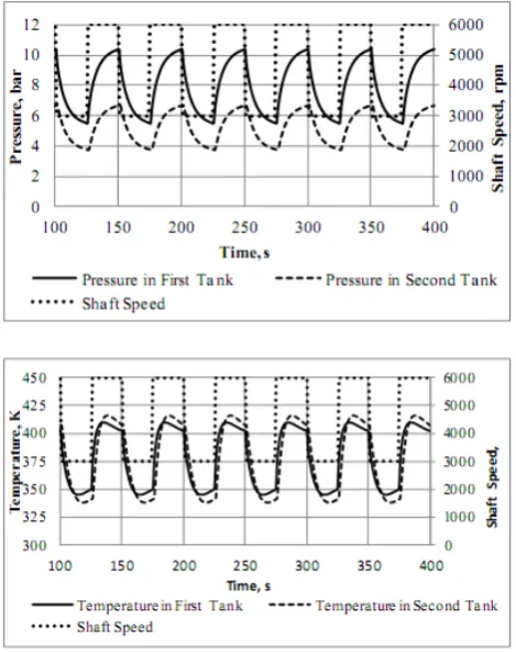
[image:11.595.61.296.280.577.2]Two diagrams presenting calculated results of dynamic response of a three tank model are presented in Figure 17. They are the pressure and temperature history as a function of a varying the shaft speed from 3000 to 6000 rpm within already developed and well established plant dynamics.
Figure 17. Pressure (up) and temperature (below) in three tanks while changing speed from 3000 to 6000rpm and back to 3000.
4. Conclusion
This paper gives some insight into screw compressor behaviour during start-up, as well as during variation of shaft speed, tank volume, tank pressure and throttle valve position. The experimental results presented in diagrams show such transients as speed, torque, discharge temperature and pressures for different types of the compressor start modes. The predicted results, thus obtained agree well with measured results and this data is being used as a basis for further research in developing a mathematical model
simulating screw compressor transient processes and conditions.
By including the volume of a compressor plant system, within a well proven mathematical model of a screw compressor performance, it was possible to calculate the interaction of compressors and their systems under unsteady conditions.
Thus the simulation procedure has been validated for compressor behaviour under transient operating conditions.and can be used as a useful tool for analysis of unsteady behaviour of screw compressors. Further test results are needed to check its accuracy for the prediction of whole plant performance.
Notation
A – Valve cross sectional area U – Internal energy
u – Specific internal energy u=u(θ) θ – Rotor angle of rotation
m – Mass
ṁ – Inlet or exit mass flow rate ṁ= ṁ(θ)
h – Specific enthalpy h=h(θ)
Q – Heat transfer rate between the fluid and the compressor
surroundings Q=Q(θ)
p – Pressure R – Gas constant T – Temperature V – Volume of the tank
ρ – Density c – Specific heat t – Time
ω – Angular speed
γ – Specific heat ratio
μ – Orifice plate coefficient
REFERENCES
[1] Chukanova, E., Stosic, N., Kovacevic, A., Dhunput, A., 2012. Investigation of Start Up Process in Oil Flooded Twin Screw Compressors. International Compressor Engineering Conference. Purdue University.
[2] Chukanova, E., Stosic, N., Kovacevic, A., Rane, S., 2012. Identification and Quantification of Start Up Process in Oil Flooded Twin Screw Compressors. International Mechanical Engineering Congress & Exposition IMECE 2012.
[3] Fleming, J.S., Tang, Y. & You, C.X., 1996. Shutdown process simulation of a refrigeration plant having a twin screw compressor. International Journal of Refrigeration, 19(6), pp.422–428.
[5] Jun, W., Yezheng, W., 1990. Start-up and shut-down operation in a reciprocating compressor refrigeration system with capillary tubes. International Journal of Refrigeration, 13(3), pp.187–190.
[6] Krichel, Susanne V., and Oliver Sawodny, 2011. Dynamic Modeling of Compressors Illustrated by an Oil-flooded Twin Helical Screw Compressor. Mechatronics 21, pp.77–84. [7] Kovacevic, A., Stosic, N. and Smith, I.K., 2007: Screw
Compressors: Three Dimensional Computational Fluid Dynamics and Solid Fluid Interaction, Springer-Verlag Berlin Heidelberg.
[8] Kovacevic, A., Mujic, E., Stosic, N., Smith, I.K., 2007: An Integrated Model for the Performance Calculation of Screw Machines, IMechE.
[9] Li, B. & Allyene, A.G., 2010. A dynamic model of a vapor compression cycle with shut-down and start-up operations. International Journal of Refrigeration, 33(3), pp.538–552. [10] Link, R. & Deschamps, C.J., 2011. Numerical modeling of
startup and shutdown transients in reciprocating compressors. International Journal of Refrigeration, 34(6), pp.Pages 1398–1414.
[11] Ndiaye, D. & Bernier, M., 2010. Dynamic model of a hermetic reciprocating compressor in on–off cycling
operation. Applied Thermal Engineering, 30(8-9), pp.792–799.
[12] Powell, G., Weathers, B. & Sauls, J., 2006. Transient Thermal Analysis of Screw Compressors, Part I: Use of Thermodynamic Simulation to Determine Boundary Conditions for Finite Element Analyses. International Compressor Engineering Conference, Purdue University. [13] Sauls, J., Weathers, B. & Powell, G., 2006. Transient
Thermal Analysis of Screw Compressors, Part III: Transient Thermal Analysis of a Screw Compressor to Determine Rotor-to- Rotor Clearances. International Compressor Engineering Conference. Purdue University.
[14] Sauls, J., Powell, G., Weathers, B.: Thermal Deformation Effects on Screw Compressor Rotor Design, American Standard 2007.
[15] Stosic, N., Smith, I.K. and Kovacevic, A, 2005: Screw Compressors: Mathematical Modelling and Performance Calculation, Springer-Verlag Berlin Heidelberg.