Object Tracking By Online Discriminative Feature Selection Algorithm

(1)

Object Tracking By Online Discriminative Feature Selection Algorithm

Ms.Ashwini Narake

1

_{, Mrs.Pradnya Kharat}

2

_{, Ms. Rupali Ghodake}

3

1,3 _{Lecturer M.E.(ENTC), Dept. of Electronics and Telecommunication Engineering ,Agppi college, solapur,}

Maharashtra, India.

2_{Lecturer M.E.(Digital system), Dept. of Electronics and Telecommunication Engineering ,Agppi college, solapur}

Maharashtra, India.

---*---Abstract -**

Most tracking-by-detection algorithms train

discriminative classifiers to separate target objects from their surrounding background. In this setting, noisy samples are likely to be included when they are not properly sampled, thereby causing visual drift. The multiple instances learning (MIL) learning paradigm has been recently applied to alleviate this problem. However, important prior information of instance labels and the most correct positive instance (i.e., the tracking result in the current frame) can be exploited using a novel formulation much simpler than an MIL approach. In this paper, it shows that integrating such prior information into a supervised learning algorithm can handle visual drift more effectively and efficiently than the existing MIL tracker. It present an online discriminative feature selection algorithm which optimizes the objective function in the steepest ascent direction with respect to the positive samples while in the steepest descent direction with respect to the negative ones. Therefore, the trained classifier directly couples its score with the importance of samples, leading to a more robust and efficient tracker. Numerous experimental evaluations with state-of-the-art algorithms on challenging sequences demonstrate the merits of the proposed algorithm.

Keywords: steepest ascent, steepest descent, optimize, Robust, trained classifier.

1. Introduction

Object tracking has been extensively studied in computer vision due to its importance in applications such as automated surveillance, video indexing, traffic monitoring, and human-computer interaction, to name a few. While numerous algorithms have been proposed during the past decades, it is still a challenging task to build a robust and efficient tracking system to deal with appearance change caused by abrupt motion, illumination variation, shape deformation, and occlusion .It has been demonstrated that an effective adaptive appearance model plays an important role for object tracking .

A simple and effective online discriminative feature selection (ODFS) approach which directly couples the classifier score with the sample importance, thereby formulating a more robust and efficient tracker than state-of-the-art algorithms and 17 times faster than the MIL Track method (both are implemented in MATLAB).

It is unnecessary to use bag likelihood loss functions for feature selection as proposed in the MIL Track method. Instead, it can directly select features on the instance level by using a supervised learning method which is more efficient and robust than the MIL Track method. As all the instances, including the correct positive one can be labeled from the current classifier, they can be used for update via self-taught learning. Here, the most correct positive instance can be effectively used as the tracking result of the current frame in a way similar to other discriminative models.

2. Problem Statement

Most tracking by detection algorithms train discriminative classifier to separate target object from their surrounding background .In this setting ,noisy samples are likely to be included when they are not properly sampled their by causing visual drift . Our proposed work is to;

 Design an algorithm to eliminate this problem.

 To analyze our tracker performance with numerous experimental results and evolutions on challenging video or image sequences in terms of efficiency, accuracy and robustness.

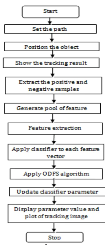
3. Theoretical Framework

Block diagram of tracking:

Fig3.1: Block Diagram of Tracking Sample

Set of Image patches

Track Location

Feature Extractio n

Select

Feature

Apply classifier to each feature vector Apply

ODFS algorith m Update

(2)

Figure illustrates the basic flow of algorithm. The discriminative appearance model is based a classifier which estimates the posterior probability given a classifier, the tracking by detection process is as follows. Let the location of sample at frame. The object location where assume the corresponding sample and then densely crop some patches within a search radius centering at the current object location and label them as positive samples. Then, randomly crop some patches from set and label them as negative samples. It utilizes these samples to update the classifier. When the frame arrives, it crop some patches with a large radius surrounding the old object location frame.

Next, apply the updated classifier to these patches to find the patch with the maximum confidence. The location is the new object location in the frame. Based on the newly detected object location, tracking system repeats the above mentioned procedures.

 Assume the‘t’ frame arrives crop some patches at radius alpha (α) is considered as positive samples.  Again we crop some patches randomly from set where radius is α<ς<β is considered as negative samples.

 α= 4ς= [2α] &β=[1.5α] for t-th frame.  Next we again crop some patches at radius

ς (gamma)= 25 when (t+1)th frame arrives.  Like this generate two set of image patches.  Find the tracking location with help of It (x) € R2_i.e

by calculating radius of 4 pixel.

3.2 Haar like feature extraction:

Fast computation of Haar-like features: One of the contributions of Viola and Jones was to use summed area tables, which they called integral images. Integral images can be defined as two-dimensional lookup tables in the form of a matrix with the same size of the original image. Each element of the integral image contains the sum of all pixels located on the up-left region of the original image (in relation to the element's position). This allows computing sum of rectangular areas in the image at any position or scale using only four lookups:

Fig3.2: Finding the sum of the shaded rectangular area Sum=I(C) +I (A)-I (B)-I (D).

Where points A, B,C,D belong to the integral image I, as shown in the figure. Each Haar-like feature may need more than four lookups, depending on how it was defined. Viola and Jones's 2-rectangle features need six lookups, 3-rectangle features need eight lookups, and 4-3-rectangle features need nine look ups .Lien hart and Maydt introduced the concept of a tilted (45°) Haar-like feature. This was used to increase the dimensionality of the set of features in an attempt to improve the detection of objects in images. This was successful, as some of these features are able to describe the object in a better way. For example, a 2-rectangle tilted Haar-like feature can indicate the existence of an edge at 45°.Messom and Barczak extended the idea to a generic rotated Haar-like feature. Although the idea sounds mathematically sound, practical problems prevented the use of Haar-like features at any angle. In order to be fast detection algorithms use low resolution images causing rounding errors. For this reason rotated Haar-like features are not commonly used.

3.3 Classifier Construction and Update:

In this sample is represented by a feature vector where each feature is assumed to be independently distributed as MILTrack and then the classifier can be modeled by A Naive Bayes classifier is a weak classifier with equal prior. Next, the classifier is a linear function of weak classifiers and uses a set of Haar-like features (15) to represent samples. The conditional distributions and in the classifier are assumed to be Gaussian distributed as the MIL Track method with four parameters. The parameters are incrementally estimated and N is the number of positive samples. In addition update and with similar rules. It can be easily deduced by maximum likelihood estimation method where learning rate to moderate the balance between the former frames and the current one.It should be noted that parameter update method is different from that of the MIL Track method and it can be update equations are derived based on maximum likelihood estimation. For online object tracking, a feature pool with M > K features is maintained. As demonstrated in online selection of the discriminative features between object and background can significantly improve the performance of tracking. The objective is to estimate the sample with the maximum confidence from as with K selected features. However, directly select K features from the pool of M features by using a brute force method to maximize the computational complexity with combinations is prohibitively high (set K = 15 and M = 150 in experiments) for real-time object tracking. An efficient online discriminative feature selection method which is a sequential forward selection method where the number of feature combinations is MK, thereby facilitating real-time performance.

Hk=log( kk=1p(fk(x)|y=1)P(y=1))/ ( kk=1p(fk(x)|y=0)P(y=0))=∑kk=1 (x), Where

(3)

f(x).

 Y= binary variable of gray scale image having value [0,1] .i.e. 0= black ,1=white it is y axis of image patch  Weal classifier is phi of k.

It is estimate the posterior probability i.e. confidence map function of feature vector

C(x) =P(y=1|X) = (hk(X),

 X=sample set, Sigma=sigmoid function. (Z)=1/1+e-Z

 Confidence map function is Gaussian distributed .It is plot of expected value to the variance.

3.4 Bag Likelihood with Noisy-OR Model:

The instance probability of the MIL Track method is modeled by i indexes the bag and j indexes the instance in the bag, and is a strong classifier. The weak classifier is computed by and the bag probability based on the Noisy-OR model. The MIL Track method maintains a pool of M candidate weak classifiers and selects K weak classifiers from this pool in a greedy manner using the following criterion. Each weak classifier is composed of a feature is the bag likelihood function and it is a binary label. The selected K weak classifiers construct the strong classifier as .The classifier is applied to the cropped patches in the new frame to determine the one with the highest response as the most correct object location. It show that it is not necessary to use the bag likelihood function based on the Noisy-OR model for weak classifier selection and it can select weak classifiers by directly optimizing instance probability via a supervised learning method as both the most correct positive instance (i.e. the tracking result in current frame) and the instance labels are assumed to be known.

3.5 Principle of ODFS:

The confidence map of a sample being the target is computed, and the object location is determined by the peak of the map. Providing that the sample space is partitioned into two regions it defines a margin as the average confidence of samples in minus the average confidence of samples. In the training set, assume the positive set consists of N samples and the negative set is composed of L samples. Each sample is represented by a feature vector. A weak classifier pool is maintained using objective is to select a subset of weak classifiers from the pool which maximizes the average confidence of samples in while suppressing the average confidence of samples. Therefore, maximize the margin function use a greedy scheme to sequentially select one weak classifier from the pool to maximize. A classifier constructed by a linear combination of the first weak classifiers. Note that it is difficult to find a closed form solution of the objective function in Furthermore, although it is natural and easy to directly select that maximizes

objective function in the selected is optimal only to the current samples, which limits its generalization capability for the extracted samples in the new frames. An approach similar to the approach used in the gradient boosting method to solve which enhances the generalization capability for the selected weak classifiers. The steepest descent direction of the objective function of in the (N+L) dimensional data space at the inverse gradient (i.e., the steepest descent direction) of the posterior probability function, its generalization capability is limited.

Friedman proposes an approach to select that makes most parallel to when minimizing objective function in.The selected weak classifier is most highly correlated with the gradient over the data distribution, thereby improving its generalization performance. In this work, instead select that is least parallel to as maximize the objective function. Thus, choose the weak classifier with the following criterion which constrains the relationship between Single Gradient and Single weak Classifier (SGSC) output for each sample. However, the constraint between the selected weak classifier and the inverse gradient direction is still too strong in because is limited to the small pool.

(4)

 Extract the features with these two sets of samples by the ODFS algorithm.

 ODFS algorithm use center location error in pixel to quantitatively compare which is calculated by the Gaussian distribution plot of frame per second to the position of error pixel.

Fig3.5: Gaussian distribution plot of frame per second to the position of error pixel.

3.7 Relation to Bayes Error Rate:

In this the optimization problem in is equivalent to minimizing the Bayes error rate in statistical classification. The Bayes error rate is the class conditional probability density function and describes the prior probability. In experiments, the samples in each set are generated with equal probability i.e., maximizing the proposed objective function is equivalent to minimizing the Bayes error rate.

4. Architectural Design:

4.1 Algorithm:

Algorithm1: Object tracking algorithm:

1. Input: video frame.

2. Sample a set of image patches. 3. Track the location at the frame. 4. Extract feature for each sample. 5. Apply classifier to each feature vector. 6. Find tracking location.

7. Sample two set of image patches.

8. Extract feature with these two sets of samples by the ODFS algorithm and update classifier parameters.

9. Output: tracking location and classifier parameter.

Algorithm2: Feature selection algorithm:

1. Input: dataset.

2. Update weak classifier pool.

3. Update the average weak classifier outputs. 4. Update inverse gradient.

5. Correlate gradient and classifier.

6. Calculate average weak classifier output. 7. Normalize classifier.

8. Output : strong classifier and confidence map function.

ODFS tracker selects 15 features for classifier construction which is much more efficient than the MIL Track method that sets K = 50. The number of candidate features M in the feature pool is set to 150, which is fewer than that of the MIL Track method (M = 250).Use radius of 4 pixels for cropping the similar positive samples in each frame and generate 45 positive samples. A large can make positive samples much different which may add more noise but a small generates a small number of positive samples which are insufficient to avoid noise. The inner and outer radii for the set that generates negative samples are set.

Set the inner radius larger than the radius to reduce the overlaps with the positive samples which can reduce the ambiguity between the positive and negative samples. We use the same generalized Haar-like features as which can be efficiently computed using the integral image. Each feature fk is a Haar-like feature computed by the sum of weighted pixels in 2 to 4 randomly selected rectangles. For presentation clarity, in we show the probability distributions of three selected features by our method. The positive and negative samples are cropped from a few frames of a sequence. The results show that a Gaussian distribution with an online update using is a good approximation of the selected features. As the proposed ODFS tracker is developed to addresses issues of MIL based tracking methods. We evaluate it with the MIL Track on 16 challenging video clips, among which 14 sequences are publicly available and the others are collected on our own. In addition, seven other state-ofthe-art learning based trackers are also compared. For fair evaluations, we use the original source or binary codes in which parameters ofeach method are tuned for best performance. The 9 trackerswe compare with are: fragment tracker (Frag), online AdaBoost tracker (OAB) ,Semi-Supervised Boosting tracker(SemiB) ,multiple instance learning tracker (MILTrack) Tracking-Learning detection(TLD)method, Struck method 1-tracker visual tracking decomposition(VTD) method and compressive tracker (CT) .We fix the parameters of the proposed algorithm for all experiments to demonstrate its robustness and stability. Since all the evaluated algorithms involve some random sampling except we repeat the experiments 10 times on each sequence, and present the averaged results. Implemented in MATLAB, our tracker runs at 30 frames per second (FPS) on a Pentium Dual-Core 2:10 GHz CPU with 1:95 GB RAM.

(5)

set as 8 and 38, respectively. Note that we set the inner radius larger than the radius to reduce the overlaps with the positive samples, which can reduce the ambiguity between the positive and negative samples. Then, we randomly select a set of 40 negative samples from the set X, which is fewer than that of the MIL Track method (where 65 negative examples are used). Moreover, we do not need to utilize many samples to initialize the classifier whereas the MIL Track method uses 1000 negative patches. The radius for searching the new object location in the next frame is set as = 25 that is enough to take into account all possible object locations because the object motion between two consecutive frames are often smooth, and 2000 samples are drawn, which is the same as the MIL Track method.

Therefore, this procedure is time-consuming if we use more features in the classifier design. Our ODFS tracker selects 15 features for classifier construction which is much more efficient than the MIL Track method that sets K = 50. The number of candidate features M in the feature pool is set to 150, which is fewer than that of the MIL Track method (M = 250). We note that we also evaluate with the parameter settings K = 15; M = 150in the MILTrack method but find it does not perform well for most experiments. The learning parameter can be set as 0.80 to 0.95. A smaller learning rate can make the tracker quickly adapts to the fast appearance changes and a larger learning rate can reduce the likelihood that the tracker drifts off the target. Good results can be achieved by fixing 0.93in our experiments.

4.2 Experimental set up and results

All of the test sequences consist of gray-level images and the ground truth object locations are obtained by manual labels at each frame. We use the center location error in pixels as an index to quantitatively compare 10 object tracking algorithms. In addition, we use the success rate to evaluate the tracking results This criterion is used in the PASCAL VOC challenge and the score is defined as score = area (Intersection)/area (G union T), where G is the ground truth bounding box and T is the tracked bounding box. If score is larger than 0.5 in one frame, then the result is considered a success. Shows the experimental results in terms of center location errors, and presents the tracking results in terms of success rate. Our ODFS based tracking algorithm achieves the best or second best performance in most sequences, both in terms of success rate and center location error. Furthermore, the proposed ODFS based tracker performs well in terms of speed (only slightly slower than CT method) among all the evaluated algorithms on the same machine even though other trackers (except for the TLD, CT methods and `1-tracker) are implemented in C or C++ which is intrinsically more efficient than MATLAB. We also implement the MIL Track method in MATLAB which runs at 1.7 FPS on the same machine. Our ODFS-based tracker (at 30 FPS) is more than 17 times faster than the MIL Track method with more robust performance in terms of success rate and center location error. The quantitative

results also bear out the hypothesis that supervised learning method can yield much more stable and accurate results than the greedy feature selection method used in the MIL Track algorithm as we integrate known prior (i.e., the instance labels and the most correct positive sample) into the learning procedure.

4.3 Flow chart:

Fig 4.1: Flow chart of ODFS algorithm

6. Results:

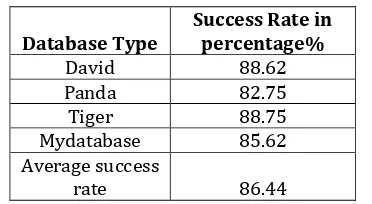
[image:5.595.345.513.181.579.2]

6.1. Result analysis table of all types of databases.

Table of success rate:-

(6)

David 88.62

Panda 82.75

Tiger 88.75

Mydatabase 85.62

Average success

[image:6.595.70.256.78.180.2]

rate 86.44

Table 6.1: Result analysis of all type databases.

Analysis table:-

The table 6.2 gives the success rate of all databases. In the table the effect like brightness, saturation, contrast and Noisy is added to database. The effect added is 10% and 90% i.e. minimum and maximum level of effect is applied and under this all effect result of database is calculated in terms of success rate given in table.

Database

type Effect applied Success rate in percentage %

Brightness 10% 85.5

Brightness 90% 81.62

Contrast 10% 85.75

My

database Contrast 90% 87.37

Saturation 10% 87.25

Saturation 90% 85

Noisy 86.87

David

Contrast 10% 75.50

Contrast 90% 88.12

Noisy 83.54

Panda

Brightness 10% 84

Contrast 10% 79.37

Contrast 90% 78.75

Saturation 90% 82

[image:6.595.306.563.116.544.2]

Noisy 83.87

Table 6.2: Result analysis of all type databases with applied effect.

Changed in predefined parameter:-

The table 6.3 gives the changed predefined parameter which is set fixed for standard database. The fixed parameter is varied from maximum to minimum. Here only one database is used i.e. (David database). And the parameter of database

is varied and success rate is calculated for each and every varied parameter.

Database

type Parameter name Values Range of values rate (%) Success

David Learning

rate Predefined value 0.93 88.62

Minimum

value 0.61 87.12

Maximum

value 0.90 88.25

David Image size Predefined

value 320x240 88.62

Minimum

value 314x235 89.75

Maximum

value 620x480 90.25

David Database

value Predefined value [120 55 75 95] 88.62 Minimum

value [100 50 70 90] 91.87 Maximum

value [200 100 90 100] 98.50

David Number of

feature pool

Predefined

value 150 88.62

Minimum

value 50 78.50

Maximum

value 200 89

David Number

selected feature

Predefined

value 15 88.62

Minimum

value 10 78.25

Maximum

value 50 92

David Searching window size

Predefined

value 25 88.62

Minimum

value 15 87.37

Maximum

value 50 92

Table 6.3: Result analysis of all type databases with changed parameter.

[image:6.595.48.276.315.652.2]

Result:- The result displays the GUI windows for different database.

[image:6.595.318.551.616.754.2]

(7)

tracking. With help of this GUI we can combine &displays all the result like tracking, plot & parameter calculation.GUI helps us to displays result combinely. The figure 6.1 gives 18 pushbotton which help us to call all the respected file and display the result with help of GUI.

Result:- The result displays the tracking ,plot and parameter value for david database.

[image:7.595.326.546.78.222.2]

#462

Fig 6.2: A tracking result of David database.

[image:7.595.73.250.197.357.2]

The figure 6.2 gives tracking result of David database after complete tracking. The red rectangle indicated as searching window. 462# indicates number of iteration. The tracking indicates with help of red window.

Fig 6.3: The plot of object tracking parameter.

[image:7.595.328.540.372.503.2]

The figure 6.3 gives tracking result of David database after complete tracking. The tracking result is displayed in terms of plot. The figure 6.3 gives plot of positive feature, histogram of positive feature, negative feature, histogram of negative feature, maximum probability, histogram of maximum probability, classifier parameter plot and histogram of classifier.

Fig 6.4: The tracking parameter value for david database.

The figure 6.4 gives parameter value like number of feature pool, number of selected feature pool , initial state i.e value of grounding box, area , score value calculated by PASCAL VOC method and success rate of david database. In figure 6.4 total time of execution is also displayed.

Result:- The result displays the tracking ,plot and parameter value for panda database.

[image:7.595.60.264.451.616.2]

#31

Fig 6.5: A tracking result of Panda database.

The figure 6.5 gives tracking result of Panda database after complete tracking. The red rectangle indicated as searching window. 31# indicates number of iteration. The tracking indicates with help of red window.

[image:7.595.314.558.594.747.2]

(8)

[image:8.595.316.555.82.233.2]

complete tracking. The tracking result is displayed in terms of plot. The figure 6.6 gives plot of positive feature, histogram of positive feature, negative feature, histogram of negative feature, maximum probability, histogram of maximum probability, classifier parameter plot and histogram of classifier.

Fig 6.7:The tracking parameter value for Panda database.

The figure 6.7 gives parameter value like number of feature pool, number of selected feature pool, initial state i.e value of grounding box, area , score value calculated by PASCAL VOC method and success rate of Panda database. In figure 6.7 total time of execution is also displayed.

Result:- The result displays the tracking ,plot and parameter value for realtime database.

[image:8.595.55.269.177.304.2]

#200

Fig 6.8: A tracking result of Real time database (My database).

[image:8.595.312.555.360.524.2]

The figure 6.8 gives tracking result of Real time database (My database) after complete tracking. The red rectangle indicated as searching window. 200# indicates number of iteration. The tracking indicates with help of red window.

Fig 6.9: The plot of object tracking parameter.

The figure 6.9 gives tracking result of Real time database (My database) after complete tracking. The tracking result is displayed in terms of plot. The figure 6.9 gives plot of positive feature, histogram of positive feature, negative feature, histogram of negative feature, maximum probability, histogram of maximum probability, classifier parameter plot and histogram of classifier.

Fig 6.10:The tracking parameter value for Real time database (My database)

The figure 6.10 gives parameter value like number of feature pool, number of selected feature pool, initial state i.e value of grounding box, area , score value calculated by PASCAL VOC method and success rate of Real time database (My database).In figure 6.10 total time of execution is also displayed.

7. Advantages & Application:

7.1 Advantages:

 Scale and pose variation .  Heavy occlusion avoided.

 Abrupt motion, rotation and blur.

[image:8.595.54.269.452.609.2]

(9)

 Automated surveillance.  Video indexing.

 Traffic monitoring.

8. Conclusion:

In online discriminative features selection (ODFS) method for object tracking which couples the classifier score explicitly with the importance of the samples. ODFS method selects features which optimize the classifier objective function in the steepest ascent direction with respect to the positive samples while in steepest descent direction with respect to the negative ones. This leads to a more robust and efficient tracker without parameter tuning. The tracking algorithm achieves real time performance with MATLAB implementation on a Pentium dual-core machine. Our ODFS-based tracker is faster than the other tracking method with more robust performance in terms of success rate. The tracker achieves favorable performance when compared with several state of the art algorithms.

References:

1. “Robust online appearance models for visual tracking,” IEEE Trans. Pattern Anal. Mach. Intell.A Jepson, D. Fleet, and T. El-Maraghi,vol. 25, no. 10, pp. 1296–1311, 2003.

2. “Support vector tracking,” IEEE Trans. Pattern Anal. Mach Intell.S. Avidan, vol. 29, no. 8, pp. 1064–1072, 2004.

3. “Online selection of discriminative tracking features,” IEEE Trans. Pattern Anal. Mach. Intell.,R. Collins, Y. Liu, and M. Leordeanu, vol. 27,no. 10, pp. 1631–1643, 2005.

4. “Real-time tracking via online boosting,” In British Machine Vision Conference,H. Grabner, M. Grabner, and H. Bischof, pp. 47–56, 2006.

5. “Semi-supervised on-line boosting for robust tracking,” In Proc. Eur. Conf. Comput. Vis.H. Grabner, C. Leistner, and H. Bischof, pp. 234–247, 2008.

6. “Robust object tracking with online multiple instance learning,” IEEE Trans. Pattern Anal. Mach. Intell. B. Babenko, M.-H. Yang, and S. Belongie, vol. 33, no. 8, pp. 1619–1632, 2011.

7. “Real-time compressive tracking,” In Proc. Eur. Conf. Comput.K. Zhang, L. Zhang, and M.-H. Yang, Vis., 2012.

8. “Real-time visual tracking via online weighted multiple instance learning,” Pattern Recognition,K. Zhang and H. Song, vol. 46, no. 1, pp. 397–411, 2013.

9. “Online selection of discriminative features using bayes error rate for visual tracking,” Advances in Multimedia Information Processing-PCM 2006,D. Liang, Q. Huang, W. Gao, and H. Yao, pp. 547–555, 2006. 6

10. “Online selecting discriminative tracking features using particle filter,” in Proc. IEEE Conf. Comput. Vis. Pattern Recognit.Y. Wang, L. Chen, and W. Gao, vol. 2, pp. 1037–1042, 2005.

11. “Gradient feature selection for online boosting,” in Proc. Int. Conf. on Comput. Vis.,X. Liu and T. Yu, pp. 1–8, 2007.

Object Tracking By Online Discriminative Feature Selection Algorithm