An Analysis on Implementation of various Deblurring Techniques in Image Processing

(1)

An Analysis on Implementation of various Deblurring Techniques in

Image Processing

M.Kalpana Devi

1

_{, R.Ashwini}

2

1,2_{Assistant Professor, Department of CSE, Jansons Institute of Technology, Karumathampatti, Coimbatore,}

Tamil Nadu, India.

---*---Abstract -**

The image processing is an important field of

research in which we can get the complete information about any image. One of the main problems in this research field is the quality of an image. So the aim of this paper is to propose an algorithm for improving the quality of an image by removing Gaussian blur, which is an image blur. Image deblurring is a process, which is used to make pictures sharp and useful by using mathematical model. Image deblurring have wide applications from consumer photography, e.g., remove motion blur due to camera shake, to radar imaging and tomography, e.g., remove the effect of imaging system response. This paper focused on image restoration which is sometimes referred to image deblurring or image deconvolution. There have been many methods that were proposed in this regard and in this paper we will examine different methods and techniques of deblurring. The aim of this paper is to show the different types of deblurring techniques, effective Blind Deconvolution algorithm and Lucy-Richardson algorithm for image restoration which is the recovery in the form of a sharp version of blurred image when the blur kernel is unknown.

Key Words: Image Deblurring, Image recovery, Blind Deconvolution, PSF,Lucy-Richardson Algorithm, Regularized filter, Wiener filter, Digital Image.

1.INTRODUCTION

In image processing world, the blur can be caused by many factors such as defocus, unbalance, motion, noise and others. In human being, the vision is one of the important senses in our body. So the image processing also plays an important role in our life. An important problem in image processing is its blurring problem which degrades its performance and quality. Deblurring is the process of removing blurring artifacts from images, such as blur caused by defocus aberration or motion blur. The blur is typically modeled as the convolution of a (sometimes space- or time-varying) point spread function(PSF) with a hypothetical sharp input image, where both the sharp input image (which is to be recovered) and the point spread function are unknown. Image deblurring is used to make pictures

sharp and useful by using mathematical model. Image deblurring (or restoration) is an old problem in image processing, but it continues to attract the attention of researchers and practitioners alike. A number of real-world problems from astronomy to consumer imaging find applications for image restoration algorithms. Image restoration is an easily visualized example of a larger class of inverse problems that arise in all kinds of scientific, medical, industrial and theoretical problems. To deblur the image, a mathematical description can be used. (If that's not available, there are algorithms to estimate the blur. But that's for another day). It can be started with a shift-invariant model, meaning that every point in the original image spreads out the same way in forming the blurry image. This model with convolution is:

g(m,n) = h(m,n)*f(m,n) + u(m,n)

(2)

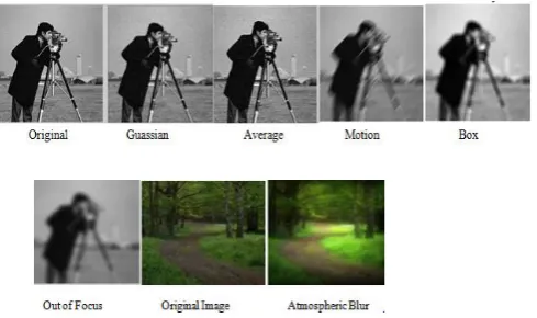
2.BLURRING TYPES

2.1 Gaussian Blur

In image processing, a Gaussian blur (also known as Gaussian smoothing) is the result of blurring an image by a Gaussian function. It is a widely used effect in graphics software, typically to reduce image noise and reduce detail. The visual effect of this blurring technique is a smooth blur resembling that of viewing the image through a translucent screen, distinctly different from the bokeh effect produced by an out-of-focus lens or the shadow of an object under usual illumination. Gaussian smoothing is also used as a pre-processing stage in computer vision algorithms in order to enhance image structures at different scales.

The Gaussian blur is a type of image-blurring filters that uses a Gaussian function (which also expresses the normal distribution in statistics) for calculating the transformation to apply to each pixel in the image. The equation of a Gaussian function in one dimension is

in two dimensions, it is the product of two such Gaussians, one in each dimension:

2.2 Average Blur

The Average blur is one of several tools you can use to remove noise and specks in an image. Use it when noise is present over the entire image. This type of blurring can be distribution in horizontal and vertical direction and can be circular averaging by radius R which is evaluated by the formula:

R =√g2_{+ f}2

where: g is the horizontal size blurring direction and f is vertical blurring size direction and R is the radius size of the circular average blurring.

2.3 Motion Blur

Motion blur is the apparent streaking of rapidly moving objects in a still image or a sequence of images such as a movie or animation. It results when the image being recorded changes during the recording of a single exposure, either due to rapid movement or long exposure.

To compute the filter coefficients, h, for 'motion'

1. Construct an ideal line segment with the desired length and angle, centered at the center coefficient of h.

2. For each coefficient location (i,j), compute the nearest distance between that location and the ideal line segment.

3. h = max(1 - nearest_distance, 0); 4. Normalize h:h = h/(sum(h(:)))

2.4 Box Blur

A box blur, (also known as a box linear filter) is a spatial domain linear filter in which each pixel in the resulting image has a value equal to the average value of its neighboring pixels in the input image. It is a form of low-pass ("blurring") filter. A 3 by 3 box blur can be written as 1/9 * determinant matrix:

Due to its property of using equal weights it can be implemented using a much simpler accumulation algorithm which is significantly faster than using a sliding window algorithm.

2.5 Out of Focus Blur

(3)

the focal length and the aperture number of the lens, and the distance between camera and object. An accurate model not only describes the diameter of the COC, but also intensity distribution within the COC.

2.6 Atmospheric Blur

It occurs due to random variations in the reflective index of the medium between the object and the imaging system and it occurs in the imaging of astronomical objects.

[image:3.595.33.278.306.451.2]

Fig -1: Different types of blurring

2.7 Point Spread Function(PSF)

Point Spread Function (PSF) is the degree to which an optical system blurs (spreads) a point of light. The PSF is the inverse Fourier transform of Optical Transfer Function (OTF).in the frequency domain ,the OTF describes the response of a linear, position-invariant system to an impulse.OTF is the Fourier transfer of the point (PSF).

3. DEBLURRING BASICS

The following equation represents the blurred or degraded image: b = Po + N where, b represents blurred image, P represents the distortion operator also called the Point Spread Function (PSF). o represents the original true image. N is additive noise, initiated during image acquisition, due to which the image gets corrupted.

The main aim of deblurring is to describe the deformation exactly by deconvolving the blurred image with the PSF model. The major need of PSF is the method of reversing the convolution effort is called as deconvolution process. Based on the complexity order, there are 4 deblurring functions which are included in the toolbox. Accepting a PSF and the blurred image are the most important arguments for all the functions.

1. Deconvwnr: The least square solution can be generated. Noise amplification can be reduced by using the gained information regarding the noise during the process of deblurring, for which the wiener filter is helpful.

2. Deconvreg: A constrained least squares solution is generated for locating the constraints on the output image. Here regularized filter is helpful for deblurring process.

3. Deconvlucy: It generates an accelerated damped Lucy-Richardson algorithm. Optimization techniques and Poisson statistics can be used for generating multiple iterations in this function. Information about the additive noise is not provided in corrupted images. 4. Deconvblind: Without the awareness of the PSF, the deblurring process can be undergone by the blind deconvolution algorithm, which gets generated by deconvblind. Along with the restored image it returns a restored PSF. The dampling and iterative model are used by this function.

Deblurring is an iterative process which considers different parameters for each iteration. This process will be continued until the received image is based on the information range which seems to be the best of the original image. Before entering into the deblurring process, preprocessing has to be performed using edge tapper function in order to keep away from “ringing” in a deblurring image.

4. DEBLURRING TECHNIQUES

(4)

[image:4.595.27.293.91.310.2]

4.1 Deblurring Images Using the Blind Deconvolution Algorithm

Blind image deblurring method is used to deblur the degraded image, without prior knowledge of the blur kernel and additive noise. The image degradation can be modeled as

where y is the degraded image, s is the sharp unknown image, b is the blur kernel and n is the noise involved. The deblurred method finds the cost function with respect to the sharp image s and the blur kernel b and is given by

here the first term i.e., the data fidelity term results from assuming that the noise is white and Gaussian, α is the regularization parameter and Ф(s) is the regularizing function which contains prior information about s. Many image deblurring methods minimize the cost function iteratively.

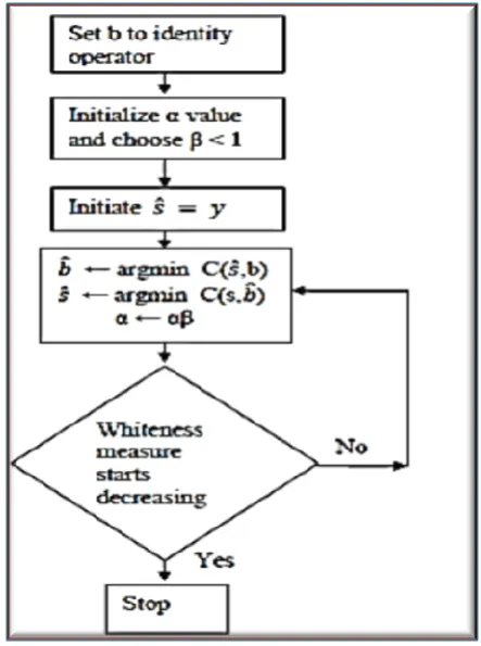
The first step involved is to set the blur kernel b to an identity operator and also to initialize the degraded image as the image estimate.

In this deblurring process, the iteration starts with a high regularization value and is gradually decreased by multiplying it with a constant β which is less than 1. Too large values of α lead to cartoon-like images or over smoothed images while too small values leads to images influenced by more noise. Based on this, the new image estimate and blur estimate are formed. The stopping criterion of this blind deblurring method corresponds to setting the final value of the regularizing parameter which is based on the whiteness measures. The cost function defined in (2) depends on the data fidelity term, the regularization value and the regularizing function Ф(s). The regularizer Ф(s) was chosen as it favors the sharp edges and also for certain values of the parameters, the prior is close to the actual observed edges. The sparse edges are quite visible in the first few iterations, but are almost unnoticeable in the final iteration. When the image to be deblurred is noisy, to prevent the appearance of the noise in the deblurred image, the final regularization cannot be made so weak.

[image:4.595.314.536.411.709.2]

(5)

effectively when no information about the distortion (blurring and noise) is known. The algorithm restores the image and the point-spread function (PSF) simultaneously. The accelerated, damped Richardson-Lucy algorithm is used in each iteration. Additional optical system (e.g. camera) characteristics can be used as input parameters that could help to improve the quality of the image restoration. PSF constraints can be passed in through a user-specified function.

The following steps are the algorithm for blind deconvolution

Step 1: Read Image Step 2: Simulate a Blur

Step 3: Restore the Blurred Image Using PSFs of various Sizes

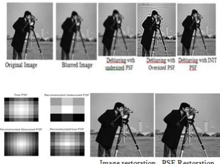
 The first restoration, J1 and P1, uses an undersized array, UNDERPSF, for an initial guess of the PSF.

 The second restoration, J2 and P2, uses an array of ones, OVERPSF, for an initial PSF that is 4 pixels longer in each dimension than the true PSF

 The third restoration, J3 and P3, uses an array of ones, INITPSF, for an initial PSF that is exactly of the same size as the true PSF. Step 4: Analyzing the Restored PSF

 The PSF reconstructed in the first restoration, P1, obviously does not fit into the constrained size. It has a strong signal variation at the borders. The corresponding image, J1, does not show any improved clarity vs. the blurred image, Blurred.

 The PSF reconstructed in the second restoration, P2, becomes very smooth at the edges. This implies that the restoration can handle a PSF of a smaller size. The corresponding image, J2, shows some deblurring but it is strongly corrupted by the ringing.

 Finally, the PSF reconstructed in the third restoration, P3, is somewhat intermediate between P1 and P2. The array, P3, resembles the true PSF very well. The corresponding image, J3, shows significant improvement; however it is still corrupted by the ringing. Step 5: Improving the Restoration

[image:5.595.310.532.249.414.2]

Step 6:Using Additional Constraints on the PSF Restoration

Fig -4: Deblurring images using Blind Deconvolution

4.2Deblurring Images Using the Lucy-Richardson Algorithm

The Lucy-Richardson algorithm can be used effectively when the point-spread function PSF (blurring operator) is known, but little or no information is available for the noise. The blurred and noisy image is restored by the iterative, accelerated, damped Lucy-Richardson algorithm. The additional optical system (e.g. camera) characteristics can be used as input parameters to improve the quality of the image restoration.

The following steps are the algorithm for Lucy-Richardson Algorihtm

Step 1: Read Image

Step 2: Simulate a Blur and Noise

(6)

4.3 Deblurring Images Using a Regularized Filter

Regularized deconvolution can be used effectively when constraints are applied on the recovered image (e.g., smoothness) and limited information is known about the additive noise. The blurred and noisy image is restored by a constrained least square restoration algorithm that uses a regularized filter.

The following steps are the algorithm for Regularized filter

Step 1: Read Image

Step 2: Simulate a Blur and Noise

Step 3: Restore the Blurred and Noisy Image Step 4: Reduce Noise Amplification and Ringing Step 5: Use the Lagrange Multiplier

[image:6.595.33.274.100.155.2]

Step 6: Use a Different Constraint

Fig -6: Deblurring images using Regularized Filter

4.4Deblurring Images Using a Wiener Filter

The Wiener filter is an important tool in image processing and it essentially performs deconvolution. The formula for the Wiener filter reduces to:

Where G(w1,w2) is the deblurred image, F(w1,w2) is the blurred image, H(w1,w2) is the blur kernel, and SNR(w1,w2) is the singal-to-noise ratio. If there is no noise then the equation reduces to:

But there are some cons of using the Wiener filter. In the representations of the images below we used deconvwnr function in MATLAB. It is noted that this function cannot recover the image perfectly, even when the noise is known. In fact, the original image can only be recovered perfectly when there is no noise and the point spread function is known. Noise has a huge impact on the quality of the recovered photo. If the image has Gaussian white noise, the Wiener filter works well when the variance is small, for example 0.00001. Another downfall of the Wiener filter is it does not work well when the point spread function is not known.

One could estimate the point spread function, but even a small change in the point spread function can lead to catastrophic results. It is noted however, if noise parameters are added to an estimated point spread function, than the results can be improved. However, these are still not ideal. In conclusion the Wiener filter is useful when the point spread function is known or can be well estimated, and a good estimation of the noise can be obtained. The issue of noise was dealt with earlier using the wavelet transform.

Wiener deconvolution can be useful when the point-spread function and noise level are known or can be estimated.

The following steps are the algorithm for Wiener filter

Step 1: Read Image.

Step 2: Simulate a Motion Blur. Step 3: Restore the Blurred Image. Step 4: Simulate Blur and Noise.

Step 5: Restore the Blurred and Noisy Image: Step 6: Simulate Blur and 8-Bit Quantization noise

[image:6.595.35.267.483.545.2]

(7)

[image:7.595.43.270.85.260.2]

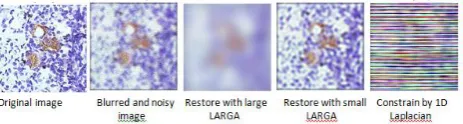
[image:7.595.329.544.320.398.2]

4.5Deblurring With Blurred/Noisy Image Pairs: In this approach the image is deblurred with the help of noisy image. As a first step both the images the blurred and noisy image are used to find an accurate blur kernel. It is often very difficult to get blur kernel from one image. Following that a residual deconvolution is done and this will reduce artifacts that appear as spurious signals which are common in image deconvolution. As the third and final step the remaining artifacts which are present in the non-sharp images are suppressed by gain controlled deconvolution process. The main advantage of this approach is that it takes both the blurred and noisy image and as a result produces high quality reconstructed image. With these two images an iterative algorithm has been formulated which will estimate a good initial kernel and reduce deconvolution artifacts. There is no special hardware is required. There are also disadvantages with this approach like there is a spatial point spread function that is invariant.

Fig - 8: Deblurring with blurred / Noisy Image

4.6 Deblurring With Motion Density Function:

[image:7.595.318.552.547.713.2]

In this method image deblurring is done with the help of motion density function. A unified model of camera shake blur and a framework has been used to recover the camera motion and latent image from a single blurred image. The camera motion is represented as a Motion Density Function (MDF) which records the fraction of time spent in each discretized portion of the space of all possible camera poses. Spatially varying blur kernels are derived directly from the MDF. One limitation of this method is that it depends on imperfect spatially invariant deblurring estimates for initialization.

Fig -9: Deblurring with Motion Density Images

4.7 Deblurring With Handling Outliers:

In this method various types of outliers such as pixels saturation and non-Gaussian noise are analysed and then a deconvolution method has been proposed which contains an explicit component for outlier modelling. Image pixels are classified into two main categories: Inlier pixels and Outlier pixels.

Fig -10: Deblurring with Motion Density Images a,b,c )Noisy and blury images d,e) Deblurred result using

[image:7.595.57.267.621.700.2]

(8)

In this approach ASDS (Adaptive Sparse Domain Selection) scheme is introduced, which learns a series of compact sub-dictionaries and assigns adaptively each localpatch a sub-dictionary as the sparse domain. With ASDS, a weighted l1-norm sparse representation model will beproposed for IR tasks. Further two adaptive regularizationterms has been introduced into the sparse representation framework. First, a set of autoregressive (AR) models are learned from the dataset of example image patches. The best fitted AR models to a given patch are adaptively selected to regularize the image local structures. Second, the image nonlocal self-similarity is introduced as another regularization term.

4.9Deblurring with Hyperspectral(PCA):

This method first uses PCA to decorrelate the HS images and separate the information content from the noise. The first k PCA channels contain most of the total energy of a HS image (i.e. most information of the HS image), and the remaining B − k PCA channels (where B is the number of spectral bands of HSI and B k) mainly contain noise. If deblurring is performed on these noisy and high-dimensional B − k PCs, then it will amplify the noise of the data cube and cause high computational cost in processing the data, which is undesirable. Therefore, we use a fast TV method with group sparsity [7] to jointly denoise and deblur only the first k PCA channels. We remove the noise (without deblurring) in the remaining PCA channels using a soft-thresholding scheme.

4.10 Deblurring with neural networks:

A multilayer neural network based on multi-valued neuron (MLMVN) .This network consist of multi-value neurons(MVN).That neuron with complex value weight and activation function , defined as a function of the argument of a weighted sum. It is based on principles of multi-valued threshold logic over the field of complex numbers formulated and development. A comprehensive observation of the discrete value

(9)

[image:9.595.61.267.81.219.2]

Propogation

5.DEBLURRING WITH KNOWN PSF

[image:9.595.321.538.216.297.2]

The performance evaluations of the deblurring operation with known PSF can be implemented by two cases: the first case has a known amount of blur, but no noise, was added to an image, and second case is a known amount of blur and noise add to the image then the image was filtered to remove this known amount of blur and noise using Wiener, regularized and Lucy-Richardson deblurring methods. In the first case the regularized and Wiener techniques produced what appeared to be the best results but it was surprising that the Lucy-Richardson technique produced the worst results in this instance.

Fig -12: Deblurring with known PSF

6.DEBLURRING WITH NO PSF INFORMATION

In this case applied with another technique is called Blind deconvolution technique which gets executed after the guess of the PSF, the number of

[image:9.595.301.563.393.660.2]

iterations and the weight threshold of it. After much experimentation, it turned out that the weight threshold should be set between 0.10 and 0.25, the PSF matrix size should be set to 13x13, and the number of iterations should be any number more than 30.In this paper the best result is got when the PSF size is 13*13, iteration is 50 and weight threshold is 0.19.

Fig -13: Deblurring with no PSF

7. COMPARISON OF DIFFERENT DEBLURRING TECHNIQUES

Table 1: Comparison Table

Method Types of blur

Performan ce

PSNR Ratio Blind

deconvolution Gaussian blur

Efficient and

good 26.77

Lucy

Richardson Gaussian blur Efficient 21.05

Wiener filter Gaussian blur Worst

performance 17.07 Regularised

filter Gaussian blur Efficient 20.12

Using MDF Motion Efficient 24.29

Using Handling

outliers Gaussian Efficient 21.92

Using ASDS-AR Gaussian Very Efficient 31.21 Neural

Networks

Gaussian

Out-of-focus Very Efficient 30.10 Hyperspectral

(PCA)

Hyperspectra

[image:9.595.57.263.496.661.2]

(10)

8. CONCLUSION AND FUTURE WORK

The review of different research papers has given the different parameters for various techniques for deblurring the image. The overall complete review is about the image quality. Many of parameters are used to improve the quality of an image. So the proposed algorithm is about the image quality. By analyzing various methods, we conclude that in the category of Non-blind methods, wiener filter give worst performance, its PSNR (peak signal to noise ratio) value is low as compared to other techniques and LR method is good, its PSNR value is high as compared to other methods. Blind deconvolution method is gives best result in comparison with non-blind techniques. ADSD-AR gives highest PSNR value. It is good because it means that the ratio of peak signal-to-noise is higher. The future work of this paper is to increase the speed of the deblurring process that is reducing the number of iteration using for deblurring the image for achieving better quality image.

REFERENCES

[1] J. P. Oliveira, M. A. T. Figueiredo, and J. M. Bioucas-Dias, “Blind estimation of motion blur parameters for image deconvolution,” in Proc. Iberian Conf. Pattern Recognit.. Image Anal., 2007, pp. 604-611.

[2] B. Amizic, S. D. Babacan, R. Molina, and A. K. Katsaggelos, “Sparse Bayesian blind image deconvolution with parameter estimation,” in Proc. Eur. Signal Process. Conf., 2010, pp. 626-630.

[3] A. M. Thompson, J. Brown, J. Kay, and D. Titterington, “A study of methods of choosing the smoothing parameter in image restoration by

regularization,” IEEE Trans. Pattern Anal. Mach. Intell., vol. 13, no. 4, pp. 326-339, Apr. 1991.

[4] L. Dascal, M. Zibulevsky, and R. Kimmel. (2008). Signal denoising by constraining the residual to be statistically noise-similar. Dept. Comput. Sci., Univ. Israel, Technion, Israel.

[5] Y. C. Eldar, “Generalized SURE for exponential families: Applications to regularization,” IEEE Trans. Sig. Process., vol. 57, no. 2, pp. 471-481, Feb. 2009.

[6] X. Zhu and P. Milanfar, “Automatic parameter selection for denoising algorithms using a no reference measure of image content,” IEEE Trans. Image Process., vol. 19, no. 12, pp. 3116-3132, Dec. 2010.

[7] M. S. C. Almeida and L. B. Almeida, “Blind and semi-blind deblurring of natural images,” IEEE Trans. Image Process., vol. 19, no. 1, pp. 36-52, Jan 2010.

[8] R. Giryes, M. Elad, and Y. C. Eldar, “The projected GSURE for automatic parameter tuning in iterative shrinkage methods,” Appl. Comput. Harmon. Anal., vol. 30, pp. 407-422, Jun. 2011.

[9] M. S. C. Almeida and L. B. Almeida, “Blind deblurring of natural images,” in Proc. IEEE Int. Conf. Acoust., Speech, Signal Process., Apr. 2008, pp. 1261-1264.

[10] Montreal, Canada, “Pattern classification by Assembling small Neural networks” IEEE Proceedings of International Joint conference on Neural networks, july 31-August4,2005.

[11] R. Kalotra, S. A. Sagar “A Review: A Novel Algorithm for Blurred Image Restoration in the field of Medical Imaging” International Journal of Advanced Research in Computer and Communication Engineering, Vol. – 3, pp. 7116-7118, 2014

[12] D. Singh, Mr. R .K Sahu“A Survey on various Image Deblurring Techniques” International Journal of Advanced Research in Computer and Communication Engineering, Vol. – 2, pp. 4736- 4739, 2013

(11)

Feedforward Neural Network based on multi-Valued Neuron”. In:B. Reusch(Ed.) computation Intelligence, Theory and Application. Advances in Soft computing.XIV,(B.Reusch-ed.),Springer-Verlag

,Berlin,Heidelberg, New York(2005)pp.599-612

[15] Aizenberg I., Moraga C., “Multilayer Feedforward Neural Network based on multi-Valued Neuron(MLMVN) and a Backpropagation Learning Algorithm”. Soft Computing(accepted),to appear: mid 2006.

[16] W. Dong, L.Zhang, R.Lukac, G.Shi, “Image Deblurring and super – resolution by adaptive spares domain selection and adaptive regularization ”.IEEE Trans. On Image Processing, Vol .20 ,no.7,pp.1838-1857,july 2011

[17] S.Cho, J.Wang, ands.Lee,,“Handling outlier in non-blind image deconvolution ,”in Proc.ICCV,2011, PP.495-502.

[18] Anju Dahiya, R.B.Dubey,“The Comparative Studing of Deblurring Techniques”Indian Journal of Applied Research ,VOL;5 ,PP.2249- 555X, 2015.

[19] Salem Saleh Al-amri and N.V.kalyankar, “A Comparative study for deblurred average blurred image”. Internatinal Journlon computer science and Engineering,vol.02, no.03, pp.731-733,2010.

[20] A. Levin, Y. Weiss, F. Durand and W. T. Freeman, "Understanding and evaluating blind deconvolution algorithms," International Conference on Computer Vision and Pattern Recognition (CVPR), pp.1964-1971,2009.

[21] Chong Sze Tong” Double Deconvolution using a Neural Network”, proceeding of 1994 International Symposium on Speech, Image Processing and Neural Networks, 13-16 April 1994, Hong Kong.

[22] ] M. P. Ekstrom, ed., Digital Image Processing Techniques (Academic, Orlando, Fla., 1984).

[23] A. Rosenfeld, A.C.Kak.,"Digital Picture Processing", (Academic, New York, 1982),Vol. 2.

[24] Dejee Singh, Mr R. K. Sahu “A survey of various image deblurring techniques”, IJARCCE vol. 2, issue 12 december 2013.

[25] M. Ben-Ezra and S. K. Nayar, “Motion-based motion deblurring,”IEEE Trans. PAMI, vol. 26, no. 6, pp. 689– 698, Jun. 2004.

[26] Lu Yuan, Jian Sun,”Image deblurring using blurry/noisy” iimage pairs” ACM.

[27] P. Subashini, M. Krishnaveni, and V. Singh. "Image Deblurring Using Back Propagation Neural Network", World of Computer Science and Information Technology Journal (WCSIT), ISSN: 2221 -0741, Vol. 1,No. 6, 277-282, 2011.

BIOGRAPHIES

I am M.Kalpana Devi and my qualification is M.C.A., M.Phil.,M.E.,. I have 12 years of experience in Academics. I Have published 5 different papers in Image Processing.

I am R.Ashwini and my qualification is M.E.,. I have 4 years of experience in Academics.

2nd Author

Photo 1’st Author