On the Computation of Extinction Time for Some Nonlinear Parabolic Equations

(1)

http://dx.doi.org/10.4236/am.2015.65071

On the Computation of Extinction Time for

Some Nonlinear Parabolic Equations

Kossadoum Ngarmadji1_{, Siniki Ndeuzoumbet}2_{, Hilaire Nkounkou}3_{, Benjamin Mampassi}4

1_{University of N’Djamena, N’Djamena, Chad} 2_{University of Moundou, Moundou, Chad} 3_{Marien Ngouabi University, Brazzaville, Congo} 4_{Cheikh Anta Diop University, Dakar, Senegal}

Email: kossbri@yahoo.fr, siniki_ndeuzoumbet@yahoo.fr, hnkounkou@yahoo.fr, mampassi@yahoo.fr

Received 16 March 2015; accepted 6 May 2015; published 7 May 2015

This work is licensed under the Creative Commons Attribution International License (CC BY).

http://creativecommons.org/licenses/by/4.0/

Abstract

The phenomenon of extinction is an important property of solutions for many evolutionary equa-tions. In this paper, a numerical simulation for computing the extinction time of nonnegative solu-tions for some nonlinear parabolic equasolu-tions on general domains is presented. The solution algo-rithm utilizes the Donor-cell scheme in space and Euler’s method in time. Finally, we will give some numerical experiments to illustrate our algorithm.

Keywords

Nonlinear Parabolic Equations, Donor-Cell Scheme, Numerical Extinction Time, General Domains

1. Introduction

There is a large number of nonlinear partial differential equations of parabolic type whose solutions for given initial data become identically nulle in finite time T. Such a phenomenon is called extinction and T is called the extinction time. For certain problems, the extinction time can be computed explicitly, but in many cases one can only know the existence of extinction time.

Since the appearance of the pioneering work of Kalashnikov [1], extinction phenomenon in nonlinear parabolic equations has been studied extensively by many authors [2] [3]. Particular emphasis has been placed on the question as to the existence of extinction time [4]-[7].

(2)

study the extinction phenomenon of solutions for some nonlinear parabolic equations.

In this work, we propose a numerical algorithm for computing the extinction time for nonnegative solutions of some nonlinear parabolic equations. Our motivation is to reproduce the extinction phenomenon of some nonlinear parabolic equations on general domains.

This paper is organized as follows. In the next section, we present the problem model and some theoretical results. A discretization of this problem is derived in Section 3, while numerical experiments are reported in Section 4 and Section 5 is devoted to concluding remarks.

2. The Model Problem

In this work, we are concerned with the following initial-boundary value problem:

( )

in

] [

0,

u _u _{F u}

t φ

∂ _{= ∆} ₋ _Ω× _∞

∂ , (1)

[ [

0 on 0,

u= ∂Ω× ∞ , (2)

( )

0 0 > 0 in

u =u Ω = Ω ∪ ∂Ω, (3) where Ω is a 2_{bounded domain with boundary} _∂Ω_,

0

u , φ and F, being given functions.

Furthermore, for any t>0 and for all u defined in Ω×

] [

0,∞ , we will set u t x

( )( ) ( )

=u t x, , x∈ Ω. Nonlinear parabolic equations of type (1) appear in various applications. In particular they are used to des- cribe a phenomenon of thermal propagation in an absorptive medium where u stands for temperature [5]. In other applications, u is a concentration and the process is described as diffusion with absorption.

The problem of determining necessary and sufficient conditions on the functions φ and F which ensure the existence of an extinction time for solutions of (1)-(3) has been considered by several authors [1] [6] [7] [12].

In this section, we state the following result:

Theorem 1 Assume that _{u C}_∈ 1

(

_{0, ;}_∞ _L2

( )

_Ω

)

_{is a nonnegative solution of the problem}₍₁₎_-₍₃₎_where_φ_and F are nondecreasing, nonnegative derivatives functions and if F

( )

0 =0, then

( )

0

lim_t _Ω u tF s sd 0

→∞

∫ ∫

=

Proof: First, let us set G u t

(

( )

)

=

_∫

₀u t( )F s s

( )

d . We have

( )

d d

u

G u F u

t

∫

Ω =

∫

Ω t . (i) Multiplying Equation (1) by F u

( )

and integrating over Ω it follows

( )

u

( ) ( )

(

( )

)

2

F u F u u F u

t φ

Ω Ω Ω

∂ ₌ _∆ ₋

∂

∫

. (ii)

On one hand thanks to regularity of functions F, φ and u, we can write

( ) ( )

d

( )

F u φ u F u φ u n s F u φ u

Ω ∆ = ∂Ω ∇ ⋅ − ∇Ω ⋅∇

∫

where n is the unit outward to ∂Ω, ds denotes an element of surface area, since u vanishes on ∂Ω and

( )

0 0

F = , we have

_∫

_∂ΩF u

( ) ( )

∆φ u n s⋅ d =0, hence

( ) ( )

( )

F u φ u F u φ u

Ω ∆ = − ∇Ω ⋅∇

∫

. (iii)

From (ii) and (iii), we deduce

( )

( ) ( )

(

( )

)

( )

(

)

2 2

2

.

u

F u F u u u F u

t

F u

φ

Ω Ω Ω

Ω

∂ _{= −} _′ _′ _∇ ₋

∂ ≤ −

∫

(3)

Since F u′

( )

≥0 and φ′

( )

u ≥0, and according to (i), we obtain

( )

(

( )

)

2

d

dt

∫

ΩG u ≤ −

∫

Ω F u . (iv) On the other hand, multiplying Equation (1) by u yields

( )

2

( )

0

u

u u u uF u

t φ

Ω Ω Ω

∂ _′

= − ∇ − ≤

∂

∫

,

which we rewrite as

2

d ₀

dt

∫

Ωu ≤ , then the application _t _u2

Ω

∫

is decreased in +_{. It then follows}

( )

(

)

2

(

( )

)

2 ₂ ₂ 0

0 , for all 0

u t u u M t

Ω ≤ Ω = Ω ≡ >

∫

. (vi)

On the other hand, the increase of F implies that

( )

₀u

( )

d

( )

₀ud

( )

G u =

_∫

F s s F u≤ ×

_∫

s uF u= , Thus

( )

_L2_{( )}

( )

_L2_{( )}

G u uF u u _Ω F u _Ω

Ω ≤ Ω ≤ ×

∫

and according to (vi) we obtain

( )

_L2_{( )}

G u M F u _Ω

Ω ≤

∫

,

This last inequality implies

( )

(

)

2

(

( )

)

₂

2

1 _{G u} _{F u}

M Ω Ω

−

_∫

≥ −

_∫

.

Then considering (iv), we deduced

( )

2

(

( )

)

2

d 1

dt

∫

ΩG u ≤ −

∫

ΩF u  ≤ −M

∫

ΩG u . (vii) Setting w t

( )

=

_∫

_ΩG u t

(

( )

)

, we obtain

( )

2

( )

2

1

w t w t

M

′ ≤ − .

This gives after integrating

( )

2

1

0 ₁

0

w t _t

w M

≤ ≤

+ .

Knowing that w

( )

0 >0. it follows w t

( )

≥0. The passage to the limit allows us to write

( )

2

1

0 lim lim ₁ 0

0

t w t t t

w M

→∞ →∞

≤ ≤ =

+ .

Finally,

( )

₀( )

( )

lim lim u t d 0

t→∞w t =t→∞

∫ ∫

Ω F s s= .

(4)

( )

p, 0, 1

F s ≥Cs ∀ > ∀ ≥s p , (4) C is a positive constant.

then the following result is easily shown.

Corollary 1 Suppose that the assumptions of the Theorem 2.1 are satisfied, and if (4) holds for p≥1, then

( )

2_{( )}

lim _L 0

t→∞ u t Ω = . (5) Indeed, for all u t

( )

solution of (1)-(3), it comes from the assumption (4) that

( ) ( )

( )

0 d 0 d

u t _p u t

C

_{∫ ∫}

_Ω s s≤

_{∫ ∫}

_Ω F s s, that gives

( )

1

0

1 u t _d

p p

u t F s s

C +

Ω Ω

+ ≤

∫

∫ ∫

.

As p+ ≥1 2, then

( )

2

0

1

0 u t p u tF s sd

C

Ω Ω

+

≤

_∫

≤

_{∫ ∫}

.

So

( )

2

0

1

0 lim lim u t d

t t

p

u t F s s

C

Ω Ω

→∞ →∞

+

≤

_∫

≤

_{∫ ∫}

,

and as a consequence of Theorem 2.1

( )

2_{( )}

lim _L 0

t→∞ u t Ω = . □ In summary, under some assumptions we know that all nonnegative solutions of (1)-(3) have extinction time as t→ ∞. We want to determine whether extinction occurs in finite time for any given φ and F.

It is well known that, in general, there is no classical solution to this nonlinear parabolic equation for arbitrary choices of φ and F. However, there are some works dealing with approximation of extinction time for solutions of (1). For example, in [13] a numerical method to approximate the solutions of (1) has been developed in the case N=1 and in [14] an algorithm based on splitting technique was derived to compute the extinction time for solutions on a rectangular domain.

In order to determine the extinction time for some φ and F, we will derive in the next section a numerical scheme based on Donor-cell scheme. Given a sufficiently small parameter >0, we would like to determine the positive real T_ >0 such that a solution u t

( )

of the problem (1)-(3) has to satisfy the above relation

( )

,

u t ≤ ∀ >t T_. (6) We shall call T satisfying (6) as the -extinction time.

3. Discretization

3.1. Discretization of the Studied Domain

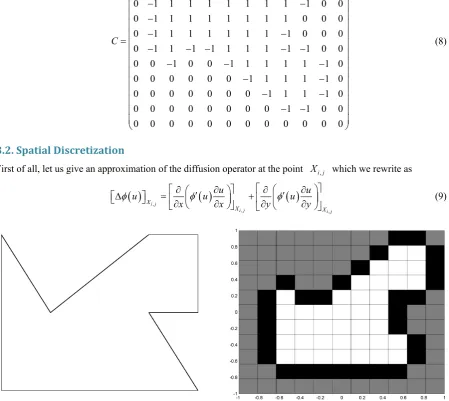
Let _{Ω ⊂}2_{be a considered domain that we assume to be of irregular shape, we approximate} _Ω_{by a domain} h

Ω whose boundary is specified by the set of boundary edges lying on gridlines. We imbed Ωh in a rectan-

gular domain Ω =R

[ ] [ ]

a b, × c d, ,

(

a b, >0

)

of smallest possible size. Given two nonzero integers imax and max

j , we set δx=

(

b a i−

)

max δy=

(

d c j−

)

max and we introduce on ΩR a grid of step δx and δy in x

and y direction respectively. The set of points

(

x yi, j

)

such that of x a i xi = + δ , yj= +c j yδ defines the discretization of ΩR into imax×jmax cells (rectangular subdomains). For all i=1, ,imax, j=1, , jmax cell

( )

i j, occupies the spatial region

[

x xi, i+1

]

× y yj, j+1 and has center the point noted Xi j, =

(

xi+1 2,yi+1 2

)

. The cells of ΩR are then divided into inner cell (which lie completely in Ω), external cell (which lie in

\ R

(5)

cells.

A matrix of size imax×jmax gives a description of the discretized domain. For example, consider three sets of

indices I, B et E corresponding to the inner, boundary and external cells, we then admit to define the following matrix

( )

1, if , ,

, 1, if , ,

0, if , .

i j I

C i j i j B

i j E ∈ 



= −_ ∈

 _∈



(7)

the matrix to identify cell types.

The idea of this numerical treatment of general domains has been suggested by Griebel et al. in [15]. An example of this numerical treatment is illustrated in Figure 1 and its matrix representative is given by the following (8).

0 0 0 0 0 0 0 0 0 0 0 0

0 0 1 1 1 1 1 1 0 0 0 0

0 1 1 1 1 1 1 1 1 1 0 0

0 1 1 1 1 1 1 1 1 0 0 0

0 1 1 1 1 1 1 1 1 1 0 0

0 0 1 0 0 1 1 1 1 1 1 0

0 0 0 0 0 0 1 1 1 1 1 0

0 0 0 0 0 0 0 1 1 1 1 0

0 0 0 0 0 0 0 0 1 1 0 0

0 0 0 0 0 0 0 0 0 0 0 0

C

 

 ₋ ₋ ₋ ₋ ₋ ₋ 

 

 − − 

 

− −

 

 ₋ 



− −



=  −_ − − − −

 − − −

 ₋ ₋



 ₋ ₋



− −

 

 

          

(8)

3.2. Spatial Discretization

First of all, let us give an approximation of the diffusion operator at the point Xi j, which we rewrite as

( )

,

, ,

i j

i j i j

X

X X

u u

u u u

x x y y

φ  ∂ φ′ ∂  ∂ φ′ ∂ 

∆ = +

  _ _ __ _ _ __

  _∂ _ _∂ _ _∂ _∂

[image:5.595.91.541.297.698.2]

     (9)

(6)

Let Vi j, be the approximation of φ

( )

u u_x ∂

 _′ 

 _∂ 

  at the cell center Xi j, . In the following we do apply a discretization that is similar to the one of Donor-cell scheme where the expression

( )

u u

x

φ ∂

 _′ 

 _∂ 

  is approached

by a progressive finite differences scheme and

( )

u u

x φ x

 ∂  _′ ∂ 

 

_∂ _ _∂ _

  by a central finite differences scheme.

Furthermore, we set φi j′, =φ′

( )

Ui j, where Ui j, ≈u X

( )

i j, and we note

(

max max max max max

)

T 0,0, , i 1,0, 0,1, , i 1,1, , 0,j 1, , i 1,j 1

φ′ φ′ ₋ φ′ φ′ ₋ φ′ ₋ φ′ ₋ ₋

Φ = (10)

If Vx denotes the vector of components Vi j, then, one can write

( )

diag p

x x

V = Φ ×D U (11) where diag

( )

Φ the diagonal matrix whose diagonal is the vector Φ and p

x

D denotes forward differentiation matrix the x-direction.

On the other hand, denoting by Wi j, the approached value of _x φ

( )

u u_x

 ∂  _′ ∂ 

 

_∂ _ _∂ _

  at the cell center Xi j, and

noting by

(

max max max max max

)

T

0,0, , 1,0, 0,1, , 1,1, , 0, 1, , 1, 1

x i i j i j

W = W W − W W − W − W − −

the vector of the value of

( )

u u

x φ x

 ∂  _′ ∂ 

 

_∂ _ _∂ _

  at point Xi j, , it follows through the central difference scheme, the

relation

c

x x x

W =D V (12) which is written by the mean of the Equation (12) as

( )

diag

c p

x x x

W =D × Φ ×D U, (13) where c

x

D denotes central differentiation matrix in the x-direction. Similarly, given Wy, the vector of the approached values of

( )

u u

y φ y

∂  _′ ∂  _∂  _∂ 

 

  at point Xi j, , we obtain

( )

diag

c p

y y y

W =D × Φ ×D U, (14) where p

y

D denotes forward differentiation matrix in the y-direction.

From Equations (13) and (14), we deduce the approximation of the operator u∆φ

( )

u at cell center Xi j, , in matrix form:

( )

(

c diag

( )

p c diag

( )

p

)

x x y y

L U = D × Φ ×D +D × Φ ×D U (15)

where L U

( )

is the vector of value of ∆φ

( )

u at points Xi j, . Thus, we have defined, an approximation operator L to approach the operator u∆φ

( )

u .

However, it should be noted that Φ is a vector dependent of U.

Considering lexicographic numerotation, we note by U t

( )

the vector of the values of u in points Xi j, ∈ Ω at time t. Knowing that u≡0 at points Xi j, ∈ Ω ΩR\ , and the differentiation matrices D D D Dxc, , , yc xp yp to approach the derivative on the set of the points Xi j, we can replace respectively by the matrices which are obtained by deleting the rows and columns corresponding to the indices of the points Xi j, of Ω ΩR\ .

Given the Equation (15), the discrete system approaching the problem (1)-(3) is rewritten by

( )

d _diag

dU Dt = × Φ U F U−

(7)

where we have set

c p c p

x x y y

D D D = × +D D ×

and where diag

( )

Φ _{is the matrix obtained of}diag

_{( )}

Φ by deleting the rows and columns corresponding to the indices of the points Xi j, of Ω ΩR\ and F U

( )

is the vector of values of F u X

(

( )

i j,

)

, Xi j, ∈ Ω. Furthermore, the initial condition is written

( )

0 0

U =U (17) where U0 is the vector obtained from U0 by deleting the elements corresponding to the indices of the points

, i j

X of Ω ΩR\

3.3. Temporal Discretization

For a time step fixed δt, we consider the sequence

( )

t_{n n}_≥₀ defined by tn+1= +tn δt et t0 =0. Then, we

denote _Un_{the approximation at time}

n

t of vector U t

( )

solution of (16)-(17). Using the explicit Euler method, the semi-discret scheme is written

( )

1

0

diag ,

0 ,

n n n n n

U U tD U tF U

U U

δ δ

+

 ₌ ₊ _× _Φ ₋

 

= 

(18)

where we set diag

( )

_{Φ =}n diag

(

_Φ

( )

_Un

)

_.

It should be noticed that if the time step δt is chosen to be little enough, and F satisfied the growth condition (4),

lim n 0

n→∞U = (19) Thus the extinction time is obtained using simple itrations process until the stopping criterion

n

U ≤_₍₂₀₎

is satisfied. Here  is the given tolerance number. The sequence of computations to be performed is sum- marized as follows

Algorithm 3.1

1. Read imax, , , jmax δt  and itermax.

2. Compute δx and δy.

3. Define ΩR (rectangular) and Ω (non rectangular) such Ω ⊂ ΩR.

4. Compute the matrix c, , , , c p p

x y x y

D D D D D_and _diag

_{( )}

Φ . 5. Set t=0, 0n= .

6. Assign initial value to U . 7. Set Uold=U0.

8. While Uold < and n<itermax, do. 9. Compute newU according to (18) . 10. Set oldU =Unew_.

11. t t= +δt n n, 1= + . End while

4. Numerical Experiments

Let Ω be a bounded domain in 2_{. Consider the initial value problem}

] [

, in 0,

q

u _{u u}

t ∂

= ∆ − Ω× ∞

(8)

[ [

0 on 0,

u= ∂Ω× ∞ (22)

( )

0 0 0 in

u =u > Ω = Ω ∪ ∂Ω. (23) where u0 is the continuous nonnegative function in Ω, vanishing on ∂Ω, and q>0.

Equation (21) models heat propagation in medium where the solution u stands for temperature.

For our numerical experiments we have consider Figure 2 to be our studied domain and we have use discretization parameters _δ_t₌₁₀−5_{, and}

max max 50

i = j = .

We would like to numerically estimate the extinction time for solutions of problem (21)-(23) with the initial condition given by

( )

(

2 2

)

0 , 1

u x y = − x +y

First, for fixed accurate value 0>0, we estimate the N-euclidian norm of the sequence Un solution of

the numerical scheme (18) for various values of parameters n. Table 1 and Figure 3 clearly show that the approximation extinction time can be given by

0 lim 0

n n

T_ = _→∞T_ (24)

We can see in Table 1 that this value is approximated by

0 0.61

T_ = (25) Also, the extinction process is illustrated by Figure 4 where we can appreciate the numerical solution extinct in a finite time.

5. Concluding Remarks

[image:8.595.172.456.411.655.2]

In this paper, a numerical algorithm based on Donor-cell scheme was proposed in order to compute the extinction time for nonnegative solutions of some nonlinear parabolic equations on general domains. We have verified

Figure 2. Discretization of studied domain Ω ⊂ −

[

1,1

] [

× −1,1

]

into cells.

Table 1.Numerical extinction time relatively to time iteration parameter n.

[image:8.595.90.531.688.724.2]

(9)

[image:9.595.140.514.193.547.2]

Figure 3. Variation norm of the numerical solution.

Figure 4. Extinction phenomenon of the numerical solution.

experimentally for a class of nonlinear parabolic equations that the numerical algorithm is efficient for computing the extinction time of solutions.

In the works to come, it will be better to apply the numerical algorithm to study, for example, moving boundary problems and extinction problems in environment.

Acknowledgements

We thank the Editor and the referee for their comments.

References

(10)

http://dx.doi.org/10.1016/0041-5553(74)90073-1

[2] Galaktionov, V.A. and Vasquez, J.L. (2002) The Problem of Blow-Up in Nonlinear Parabolic Equations. Discrete and Continuous Dynamics Systems, 8, 399-433. http://dx.doi.org/10.3934/dcds.2002.8.399

[3] Levine, H.A. (1985) The Phenomenon of Quenching: A Servey. North-Holland Mathematics Studied, 110, 275-286.

http://dx.doi.org/10.1016/S0304-0208(08)72720-8

[4] Diaz, J.I. (2001) Qualitative Study of Nonlinear Parabolic Equations: An Introduction. Extracta Mathematicae, 16, 303-341.

[5] Friedman, A. and Herrero, M.A. (1987) Extinction Properties of Semilinear HEAT Equations with Strong Absorption.

Journal of Mathematical Analysis and Applications, 124, 530-546. http://dx.doi.org/10.1016/0022-247X(87)90013-8

[6] Gu, Y.G. (1994) Necessary and Sufficient Conditions for Extinction of Solutions to Parabolic Equations. Acta Mathe-matica Sinica, 37, 73-79.

[7] Lair, A.V. (1993) Finite Extinction Time for Solutions of Nonlinear Parabolic Equations. Nonlinear Analysis, Theory,

Methods and Applications, 21, 1-8.

[8] Boni, T.K. (2001) Extinction for Dicretizations of Some Semilinear Parabolic Equations. Comptes Rendus de l’Aca- dmie des Sciences de Paris, Serie I, Mathmatique, 333, 795-800.

[9] Mikula, K.B. (1995) Numerical Solution of Nonlinear Diffusion with Finite Extinction Phenomenom. Acta Mathema-tica Universitatis Comenianae, LXIV, 173-184.

[10] Nabongo, D. and Boni, T.K. (2008) Numerical Quenching for a Semilinear Parabolic Equation. Mathematical Model-ling and Analysis, 13, 521-538. http://dx.doi.org/10.3846/1392-6292.2008.13.521-538

[11] Nabongo, D. and Boni, T.K. (2008) Quenching for Semidiscretization of a Semilinear Heat Equation with Dirichlet and Neumann Boundary Condition. Commentationes Mathematicae Universitatis Carolinae, 49, 463-475.

[12] Lair, A.V. and Oxley, M.K. (1996) Anisotropic Nonlinear Diffusion with Absorption: Existence and Extinction. Inter-national Journal of Mathematics and Mathematical Sciences, 19, 427-434.

http://dx.doi.org/10.1155/S0161171296000610

[13] Dumitrache, A. (2007) A Numerical Method to Approximate the Solutions of Nonlinear Absorption Diffusion Equa-tion. Proceeding in Applied Mathematics and Mechanics, 7, 4070041-4070042.

http://dx.doi.org/10.1002/pamm.200701050

[14] Kim, D. and Proskurowski, W. (2004) An Efficient Approach for Solving a Class of Nonlinear 2D Parabolic PDEs. In-ternational Journal of Mathematics and Mathematical Sciences, 2004, 881-899.