www.hydrol-earth-syst-sci.net/18/4277/2014/ doi:10.5194/hess-18-4277-2014
© Author(s) 2014. CC Attribution 3.0 License.
Transferring the concept of minimum energy dissipation
from river networks to subsurface flow patterns
S. Hergarten1, G. Winkler2, and S. Birk2
1Institut für Geo- und Umweltnaturwissenschaften, Albert-Ludwigs-Universität Freiburg, Freiburg i. Br., Germany 2Institut für Erdwissenschaften, NAWI Graz, Karl-Franzens-Universität Graz, Graz, Austria
Correspondence to: S. Hergarten ([email protected])
Received: 29 April 2014 – Published in Hydrol. Earth Syst. Sci. Discuss.: 4 June 2014 Revised: 28 August 2014 – Accepted: 20 September 2014 – Published: 31 October 2014
Abstract. Principles of optimality provide an interesting al-ternative to modeling hydrological processes in detail on small scales and have received growing interest in the last years. Inspired by the more than 20 years old concept of min-imum energy dissipation in river networks, we present a cor-responding theory for subsurface flow in order to obtain a better understanding of preferential flow patterns in the sub-surface. The concept describes flow patterns which are opti-mal in the sense of minimizing the total energy dissipation at a given recharge under the constraint of a given total porosity. Results are illustrated using two examples: two-dimensional flow towards a spring with a radial symmetric distribution of the porosity and dendritic flow patterns. The latter are found to be similar to river networks in their structure and, as a main result, the model predicts a power-law distribution of the spring discharges. In combination with two data sets from the Austrian Alps, this result is used for validating the model. Both data sets reveal power-law-distributed spring discharges with similar scaling exponents. These are, however, slightly larger than the exponent predicted by the model. As a further result, the distributions of the residence times strongly dif-fer between homogeneous porous media and optimized flow patterns, while the mean residence times are similar in both cases.
1 Introduction
Preferential flow due to heterogeneity is one of the most im-portant topics in subsurface hydrology. In many cases, large parts of the uncertainty in modeling subsurface flow and
transport arise from preferential flow patterns which are ei-ther not known in detail or too small-scaled to be included explicitly in the model.
Preferential flow patterns may be the result of external pre-design, but may also be created by the flow itself. Fractured aquifers and reservoirs mainly fall into the first category. Fractures may be opened at high fluid pressures (hydraulic fracturing, fluid-induced seismicity), but the basic structure of the preferential flow pattern is still governed by the geo-logic predesign here. In contrast, the role of predesign is less clear for preferential flow in soils and in karstified aquifers. In particular, the formation of conduit patterns in karst has been addressed by several modeling studies (e.g., Groves and Howard, 1994; Howard and Groves, 1995; Siemers and Dreybrodt, 1998; Kaufmann and Braun, 1999, 2000; Liedl et al., 2003; Dreybrodt et al., 2005; Kaufmann et al., 2010; Gabrovšek and Dreybrodt, 2011; Hubinger and Birk, 2011), pioneered by early work of Kiraly (1979). Although there may be some predesign, too, it is generally believed that the solution of material by the flow causes a strong tendency to-wards self-organization of the flow pattern.
The idea to explain the morphology of river networks from the concept of minimum energy dissipation is the per-haps oldest application of optimization principles in hydrol-ogy receiving considerable interest. It even dates back to the early 1990s (Howard, 1990; Rodriguez-Iturbe et al., 1992a, b; Rinaldo et al., 1992) and turned out to be rather success-ful in reproducing scale-invariant properties of drainage net-works at earth’s surface.
The probably most successful application of minimum en-ergy dissipation to flow processes so far (West et al., 1997) emerged from the field of physiology. It considers the cardio-vascular system of mammals as a space-filling hierarchical network of tubes. The principle of minimum energy dissipa-tion was shown to result in a scale-invariant structure of this network, which finally reproduces several allometric scal-ing relations found in nature. This seminal article was fol-lowed by several publications also in very prestigious jour-nals (Enquist et al., 1998, 1999; Banavar et al., 1999; West et al., 1999a, b) within a few years.
Beyond minimum energy dissipation, the minimum and maximum production of entropy are the most important vari-ational principles in nonequilibrium thermodynamics. As ex-plained, e.g., by Martyushev (2013), both are not opposed to each other, but refer to different thermodynamic constraints where maximum entropy production has a wider range of applicability. Minimum energy dissipation can also be re-lated to maximum entropy production (e.g., Županovi´c et al., 2010). So it is the most general concept of nonequilibrium thermodynamics for application to coupled or spatially dis-tributed systems in hydrology, and all the recent papers on optimization in hydrology mentioned above hinge on maxi-mum entropy production in some sense. However, maximaxi-mum entropy production is a thermodynamic principle, and delin-eating systems or subsystems that indeed act at their ther-modynamic limit and therther-modynamic constraints is nontriv-ial. As pointed out by Westhoff and Zehe (2013), finding the properties that have to be maximized or minimized in a given system is therefore still a challenge.
In this paper, we transfer the concept of self-organization towards minimum energy dissipation from river networks to subsurface flow patterns and directly derive equations for the optimal spatial distribution of porosity and permeability. In principle this is the realization of the vision on preferen-tial subsurface flow patterns described by McDonnell et al. (2007) for the case of saturated flow. A brief review on the established theory for river networks is presented in the fol-lowing section, while the more complicated theory for sub-surface flow is presented in Sect. 3.
2 The concept of minimum energy expenditure in river networks
Scale-invariant properties of river networks have been known for a long time (Horton, 1945; Hack, 1957), and the idea
to relate these properties to minimum energy dissipation (Howard, 1990; Rodriguez-Iturbe et al., 1992a, b; Rinaldo et al., 1992; Rinaldo et al., 1998) seems to be the first sub-stantial application of optimality principles in hydrology. The basic idea is that river networks organize in such a way that the total energy dissipation of the water on its way through the entire domain is minimized. So it refers to the surficial part of the water cycle starting where precipitation strikes the surface and ending when the water reaches the ocean (or any other fixed reference point).
If changes in kinetic energy are neglected, energy dissipa-tion can be computed without any knowledge of flow dynam-ics since the potential energy of the water is dissipated when it flows downslope in a channel. Then the mean energy dissi-pation (energy per time) of an individual channel segment is
P =ρgqlS, (1)
whereρis the density,gthe gravitational acceleration,qthe mean discharge (volume per time),l the length, andS the slope of the segment. In order to find those channel networks with the lowest energy dissipation (called optimal channel networks or OCNs), the domain is subdivided into discrete cells exposed to a uniform precipitation. The centers of the cells are linked by channel segments in such a way that each site (except for one or more outlet sites at the boundary) drains to exactly one neighbored site, but can be supplied by an arbitrary subset of its neighbors. This leads to dendritic river networks. The energy dissipation of the entire domain is readily obtained by summing up the contributions of all cells (Eq. 1):
P =ρgX i
qiliSi. (2)
However, minimizing P without any constraints makes no sense as the trivial solution is a flat topography where all slopes vanish, so that there is no potential energy to be dissi-pated. Therefore, the theory of OCNs introduces a constraint to the minimization ofP by assuming a relationship between slope and discharge; namely
S ∝q−θ, (3)
which makes no difference in case of uniform precipitation (minus evaporation) in the entire domain.
The OCN concept constrains the minimization of energy dissipation to steady-state topographies where homogeneous uplift is balanced by erosion, i.e., following Eq. (3). Inserting this relation into Eq. (2) leads to
P ∝X
i
liqiγ, (4)
withγ=1−θ≈0.5. This expression allows for a minimiza-tion of the energy dissipaminimiza-tion at a given uplift rate (which itself hides in the constant of proportionality) from the net-work topology alone without explicitly considering the to-pography, provided that the precipitation (minus evapora-tion) is given. In the studies on OCNs, drainage networks that minimize Eq. (4) (strictly speaking, the version without the termli that takes into account the length of the river seg-ments) were determined numerically.
It was found that these OCNs reproduce some well-known statistical properties of real river networks, such as the rela-tionship between river length and catchment size and the sta-tistical distribution of the catchment sizes, quite well. How-ever, later studies using simple erosion models (Hergarten and Neugebauer, 2001; Hergarten, 2002) revealed that some of the statistical properties can be reproduced even a little better for river networks exposed to permanently changing boundary conditions which are clearly above the minimum energy dissipation. In general, the considered statistical prop-erties of drainage networks seem to be rather robust, and it seems to be impossible to tell how close real-world river net-works are to the thermodynamic limit of minimum energy dissipation.
In the following section we transfer the concept of min-imum energy dissipation to subsurface flow. Afterwards we present two applications to different scenarios and a valida-tion using spring discharge distribuvalida-tions in order to demon-strate that the concept may be as powerful as the original minimum energy dissipation idea for river networks.
3 Theory
In the following, we assume steady-state Darcy flow of an incompressible fluid in an isotropic, but inhomogeneous porous medium with a hydraulic conductivityK(x). The vol-umetric flow rate is then given by
q(x)= −K(x)∇h(x), (5)
with the hydraulic potentialh(x). As Darcy’s law neglects ef-fects of inertia, changes in kinetic energy shall be neglected. Therefore, the potential energy of the water is completely dissipated, and the total energy dissipation per time is
P = −ρg
Z
q(x)· ∇h(x)d3x, (6)
=ρg
Z
K(x)|∇h(x)|2d3x, (7)
=ρg
Z q(x)2
K(x)d
3x, (8)
where the integral extends over the considered domain, and q(x)= |q(x)|.
The key point of this paper is determining the distribu-tion ofK(x)which minimizes the total energy dissipation. This can be either achieved by minimizing Eq. (7) with re-gard toK(x) ifh(x)is given or by minimizing Eq. (8) if q(x)is given. In principle, even a simultaneous minimization of Eq. (7) with respect to bothK(x)andh(x)can be per-formed. However, the part referring toh(x)only yields the mass balance which is shown in the following. If the spatial distribution of the conductivityK(x)is given, the fieldh(x) which minimizesP is given by the Euler–Lagrange equation of Eq. (7):
∂
∂h(x)P =div ∂
∂∇h(x)P , (9) where the derivatives are functional derivatives. This imme-diately leads to
div(K(x)∇h(x))=0, (10)
so that the distribution ofh(x)which minimizes the energy dissipation automatically satisfies the mass balance for an in-compressible fluid under saturated conditions as long as there are neither sources nor sinks. Source and sink terms can be included by taking into account the potential energy of the water entering or leaving according to its hydraulic potential. This minimization is the basis of the variational approach in finite-element groundwater modeling, but here it just illus-trates that it makes no difference whether we optimizeK(x) andh(x)simultaneously orK(x)alone and consider Darcy’s law with the mass balance separately. As the latter will be easier in the applications presented in Sect. 4, we focus on the optimization ofK(x)where eitherh(x)orq(x)is given. Similarly to the surface drainage network optimization, the optimization ofK(x)has trivial solutions, namelyP→0 if K(x)→0 everywhere (h(x)given; Eq. 7) andK(x)→ ∞
everywhere (q(x)given; Eq. 8). We thus need a constraint in analogy to the equilibrium of uplift and erosion for river networks. The idea that the total conductivity, i.e., the con-ductivity integrated over the entire domain, is given, may be straightforward at first sight. Alternatively, we can assume a given total pore space volume:
V = Z
φ (x)d3x, (11)
the second idea is more suitable because the change in V is the total amount of solid volume that has to be removed (e.g., dissolved).
In order to minimize the energy dissipation under the con-straint defined in Eq. (11), the Euler–Lagrange formalism must be applied to the functionalP−λ V instead ofPwhere the numberλis a Lagrange multiplicator. As neitherP nor V contain derivatives ofφ (x), the result is formally the same as ifφwas a parameter instead of a function:
∂
∂φ (x)P =λ ∂
∂φ (x)V . (12)
While the functional derivative on the right-hand side is al-most trivial,
∂
∂φ (x)V (φ)=1, (13)
computing the left-hand side requires a constitutive law for the conductivity as a function of the porosity, i.e., a function K(φ).
Relations between porosity and conductivity have been ex-tensively studied since the seminal work of Kozeny (1927) and Carman (1937). The original Kozeny–Carman equation predicts
K∝ φ
3
(1−φ)2, (14)
where the factor of proportionality includes a spatial length scale and the denominator becomes important in case of very high porosities. As the length scale may change if conduits are widened, applying Eq. (14) without further considera-tions may be misleading. So let us first consider the simple case of parallel tubular conduits of given radii ri. Accord-ing to the Hagen–Poiseuille law, the total conductivity of this system is
K∝X
i
ri4, (15)
while φ∝X
i
ri2. (16)
The relation between porosity and conductivity depends on how additional pore space is distributed among the conduits. Increasing all radii by the same factorβ is perhaps the sim-plest concept. Thenφincreases by a factorβ2, whileK in-creases by a factorβ4, resulting in a relationK∝φ2.
However, spending all additional pore space volume for widening the largest conduit is most efficient with regard to the conductivity. In this case we obtain
∂logK ∂logφ =
φ K
∂K ∂φ =
φ K
∂K ∂rmax
∂φ ∂rmax
= P
i ri2
P
i ri4
4r3 max 2rmax =2
P
i ri2rmax2
P
i ri4
≥2, (17)
which means that the slope in a double-logarithmicK–φplot is 2 or larger. It approaches the value of 2 obtained for widen-ing all conduits by the same factor if either all conduits are equally sized or if the largest conduit is much larger than the rest. So the relationship between conductivity and porosity is not an overall power law, but behaves like a power law with n=2 over a range of values, while it may increase faster in other regimes. Therefore, an overall power-law relationship,
K(φ)=aφn, (18)
with n≥2 seems to be the best tradeoff between a good approximation and keeping the following considerations as simple as possible. However, most of the results obtained in the following only requiren >1, which just means that the conductivity increases more rapidly than the porosity. For simplicity, we neglect the strong increase in conductivity due to the coalescence of conduits forφ→1 reflected in the de-nominator of Eq. (14).
Inserting the expression for the energy dissipation (Eq. 7), the K–φ relationship (Eq. 18), and Eq. (13) into Eq. (12) yields
ρganφ (x)n−1|∇h(x)|2=λ. (19) The Lagrange multiplicator can be eliminated using the total pore space volumeV (Eq. 11), leading to
λ=ρgan V
R
|∇h(x)|−n−21d3x
!n−1
, (20)
and finally to
φ (x)=V |∇h(x)|
−n−21 R
|∇h(ξ)|−n−21d3ξ
. (21)
So the optimal distribution of the porosity ifh(x)is given is proportional to|∇h(x)|−n−21, while the rest of Eq. (21) is
just a normalization to maintain the given total pore space volumeV.
Minimizing the energy dissipation ifq(x)is given is sim-ilar. Computing the functional derivative of Eq. (8) leads to the condition
−ρgnq(x)
2
The Lagrange multiplicator can again be eliminated using the total pore space volume according to
λ= −ρgn
a
R
q(x)n+21d3x
V
!n+1
, (23)
finally leading to
φ (x)=V q(x)
2
n+1
R
q(ξ)n+21d3ξ
. (24)
This dependency is not only similar to that obtained for the case thath(x)is given (Eq. 21), but even basically the same. This becomes obvious if we transform Eq. (21) to conductiv-ities, leading to
K(x)=aVn |∇h(x)|
−n2−n1 R
|∇h(ξ)|−n−21d3ξ
n, (25)
∝ |∇h(x)|−n2−n1. (26)
Applying the same to Eq. (24) leads to
K(x)=aVn q(x)
2n n+1
R
q(ξ)n+21d3ξ
n, (27)
∝q(x)n2+n1. (28)
Replacingq(x)withK(x)|∇h(x)| in Eq. (28), it is recog-nized that Eqs. (26) and (28) are equivalent.
Thus, the optimal distribution of porosities and conductiv-ities with respect to minimum energy dissipation is the same forh(x)given and forq(x)given and can be summarized in the following relations:
φ (x)∝ |∇h(x)|−n−21 ∝q(x)n+21, (29)
K(x)∝ |∇h(x)|−n2−n1 ∝q(x)n2+n1. (30)
In principle, we can now insert this result into the mass balance of Darcy’s law (Eq. 10) and obtain the highly non-linear differential equation
div|∇h(x)|−n2−n1∇h(x)=0. (31) However, we should keep in mind that this is a Darcy equa-tion where the conductivity increases even more than linearly with the flow rate. This results in a strong tendency to focus flow, so that this equation will not have a unique, regular so-lution in general. For this reason we refrain from considering this equation in detail here.
Beyond this, the resulting optimal distribution ofK(x)can be used to represent the total energy dissipation as a function
of eitherh(x)orq(x)alone. Plugging Eq. (25) into Eq. (7) yields
P = ρgaV
n
R
|∇h(x)|−n−21d3x
n−1. (32)
Thus, minimizing the total energy dissipation is equivalent to maximizing the functional
F (h)= Z
|∇h(x)|−n−21d3x. (33)
It is easily recognized that Eq. (31) is the Euler–Lagrange equation of this functional. As a consequence, maximizing F (h)approximately among a set of functions obeying some regularity should also provide an approximate solution of the nonlinear Darcy flow problem posed in Eq. (31).
An equivalent functional with regard toq(x)is obtained by inserting Eq. (27) into Eq. (8), resulting in
P = ρg
aVn
Z
q(x)n+21d3x
n+1
. (34)
Therefore, minimizing P is equivalent to minimizing the functional
G(q)= Z
q(x)n+21d3x. (35)
This functional will be used in the application presented in Sect. 4.2.
4 Applications
4.1 Radial flow towards a spring
Let us now determine the optimal distribution of the trans-missivity for the radially symmetric case. For a domain of radiusRwith uniform recharge, the volumetric flow rate is
q(r)∝ R
2−r2
r , (36)
where the dominator increases towards the spring due to in-creasing catchment size, and the denominator decreases due to decreasing cross-section area. From Eqs. (29) and (30) we immediately obtain
φ (r)∝
R2−r2 r
2
n+1
(37)
∝r−n+21 forr R, (38)
so that
K(r)∝r−n2+n1 forr R. (39) This leads to
∂ ∂rh(r)=
q(r) K(r)∝
r−1
r−n2+n1
=rnn−+11, (40)
and thus
h(r)∝rn2+n1 (41)
close to the spring (rR) ifh(0)=0. For all valuesn >1, the predicted increase inK(r)even overcompensates the de-crease in cross-section area towards the spring, so that the hydraulic gradient even tends to zero when approaching the spring. As discussed in Sect. 3,nshould at least be 2 in natu-ral aquifers, so that the optimalK(r)should increase at least liker−43 towards the spring, andh(r)should decrease at least
liker43.
4.2 Dendritic flow patterns
We now come to the direct analog of the optimal channel network approach reviewed in Sect. 2. As stated at the end of Sect. 3, minimizing the energy dissipation causes a ten-dency to focus flow, so that it makes sense to assume that each site in a discrete system only drains towards one of its neighbors. This topology is obvious for large-scale surface river networks except for situations where sediment deposi-tion is important, e.g., braided rivers and river deltas where flow paths may indeed split up in downstream direction. The following argument shows that splitting up the flow of a site is energetically unfavorable for subsurface flow, too. Let us assume an arbitrary network of flow paths connecting dis-crete sites with any of their neighbors. For such a disdis-crete network, the functional to be minimized (Eq. 35) turns into that for river networks (Eq. 4):
G(q)=X
i
liqiγ, (42)
with γ= 2
n+1. (43)
Let us assume that the discharges qi describe the config-uration with the minimum energy dissipation. If this con-figuration contains any site that drains towards more than one neighbor, there must be a set of configurations with dis-chargesqi+ δ qi that is allowed within a range ofaround zero. The condition that the functionalG(q+ δ q) has a minimum at=0 requires
∂2
∂2G(q+δq)
=0
>=0, (44)
but computing the second derivative immediately yields ∂2
∂2G(q+δq)
=0
=γ (γ−1)X i
li(δqi)2qγ
−2
i <0 (45) for 0< γ <1. So the original configuration with discharge towards more than one neighbor cannot be a minimum of the energy dissipation. As a consequence, nondendritic maze cave structures are not optimal in the sense of energy dissipation.
We therefore consider only dendritic networks where each site has a unique flow direction towards one of its neigh-bors, in analogy to the theory of OCNs. Similarly to this ap-proach, we focus on two-dimensional flow patterns in plan view. We subdivide the domain into square cells where each cell is exposed to the same recharge and assume that each cell drains to one of its eight nearest and second-nearest neigh-bors. Darcy’s law is only applied in one dimension along the dendritic network, while arbitrary flow directions not neces-sarily related to a hydraulic gradient are allowed.
Figure 1. Dendritic flow patterns obtained by numerical optimiza-tion for different values ofnon lattices of 4096×4096 sites. Only flow paths with a discharge of at least 10−5of the total recharge are plotted. The line width is proportional to the third root of the discharge, which is proportional to the diameter of the conduits for
n=2.
Figure 1 shows four realizations on lattices of 4096×4096 sites where outflow is allowed across the entire boundary. As expected, dendritic network structures occur for all values ofnconsidered here. The tendency towards highly branched networks increases withn. Vice versa, a significant tendency towards the shortest way to the boundary is visible forn=4
3. However, this value is outside the range n≥2 obtained for reasonable relations between porosity and permeability, but will become relevant for the discussion on turbulent flow in Sect. 5. As mentioned above,nshould not be much greater than 2, while the typical value γ=0.5 (Eq. 4) for surface river networks corresponds to n=3 according to Eq. (43). Therefore, our model predicts that the tendency to search the shortest way to the boundary should be slightly stronger for two-dimensional subsurface flow patterns than for rivers at the surface. However, it was already pointed out by Rinaldo et al. (1998) that such small variations in γ do not result in significant differences in the statistical properties of the networks.
As little is known about the internal structure of real sub-surface flow patterns, spring discharges provide the most eas-ily accessible information. Figure 2 shows that the distribu-tion of the spring dischargesQis a power law described by the probability density:
f (Q)=Q−τ, (46)
10-10 10-8 10-6 10-4
10-2 100
100 101 102 103 104 105 106 107
Probability density f(Q)
Discharge Q homogeneous / n = 1 power law with τ = 1.5
n = 4/3 n = 2 n = 3 n = 4
Figure 2. Probability density of the spring discharges of the flow patterns shown in Fig. 1 measured along the boundaries of the do-main. Discharges are scaled by assuming a unit recharge at each site, so that the discharge is the same as the number of sites in the re-spective catchment. The estimated discrete values were obtained by logarithmic binning with five bins per decade. The distributions for homogeneous porosity and forn=1 are identical and correspond to straight flow lines towards the boundary.
with τ=1.5. Transformed to a cumulative distribution, i.e., the number N (Q)of springs with a discharge greater than or equal toQ, it says
N (Q)=Q−0.5. (47)
This result is insensitive tonat least in the rangen≥4
3 con-sidered here, and thus for all reasonable relations between porosity and permeability as discussed above.
4.3 Validation
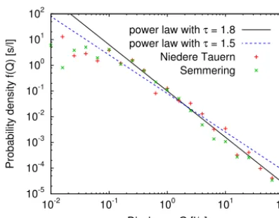
In the following we attempt to validate our model by two data sets of spring discharges from Austria. The first data set com-prises the discharges of 1675 springs in the Niedere Tauern Range, and the second one the discharges of 1001 springs in the Semmering region. The methods of data acquisition range from simple estimates to direct capture and tracer di-lution techniques. The frequency of measurement also varies from spring to spring. Despite the potential errors in the in-dividual spring discharges, both data sets reveal clear power-law distributions of the discharges above a minimum value of about 0.1 L s−1(Fig. 3). This result suggests that the sub-surface flow patterns in the two regions are indeed strongly organized.
[image:7.612.49.287.65.301.2]10-5
10-4
10-3
10-2
10-1
100
101
102
10-2 10-1 100 101 102
Probability density f(Q) [s/l]
Discharge Q [l/s]
power law with τ = 1.8
power law with τ = 1.5
[image:8.612.66.265.64.219.2]Niedere Tauern Semmering
Figure 3. Probability density of the spring discharges of the two considered data sets from Austria. The estimated discrete values were obtained by logarithmic binning with five bins per decade.
difficult. Starting a power-law fit at a minimum discharge of 0.1 L s−1even yieldsτ <1.5, but visually, the data still sug-gestτ >1.5 in these two regions.
However, the occurrence of an organized flow pattern does not imply that it is indeed self-organized. And even if it is, it does not prove that this self-organization follows the prin-ciple suggested in this study. If the prinprin-ciple of minimizing energy dissipation holds here, the deviations in the scaling exponent may, e.g., arise from a three-dimensional flow or-ganization or from the location of the springs in relation to the topography. On the other hand, the power-law distribu-tion might also be the result of a scale-invariant tectonic pre-design and not be related to any self-organization in the flow pattern. Therefore, more data sets are needed to validate or refute our idea of subsurface flow organization.
4.4 Residence time distributions
Residence times and their statistical distributions are among the most important properties in subsurface hydrology. On the one hand, they reveal valuable information about storage and flow pathways, and on the other hand they are essential for predicting the propagation of pollutants and recovery.
The spatial distribution of porosity and conductivity has a strong influence on the residence time distribution in a catch-ment. The residence time distribution is obtained by integrat-ing v(1x) over the flow path from each point of the catchment to the spring. Here,
v(x)=q(x)
φ (x) (48)
denotes the flow velocity. Using Eq. (24) we obtain
v(x)=q(x) n−1
n+1Rq(ξ)n+21d3ξ
V , (49)
∝q(x)nn−+11. (50)
Thus, the flow velocity increases with increasing flow rate for all valuesn >1. However, the increase is weaker than the linear increase occurring in a homogeneous aquifer. The exponent in Eq. (50) amounts to one-third forn=2, which means that one-third of an increase in flow rate is due to an increase in velocity, while two-thirds arise from the increase of conductivity.
At this point it should be mentioned that the residence time distribution obtained this way describes only the contribution of the flow paths since it is assumed that the entire water in a representative volume moves exactly at the velocity defined by Eq. (48). Effects of dispersion and the properties of spe-cific tracers (e.g., sorption) must be taken into account addi-tionally when making a prediction.
The relationship between flow rate and flow velocity is the perhaps most important difference of our model of subsur-face flow towards rivers at the sursubsur-face. Although the theory reviewed in Sect. 2 does not account for flow velocities ex-plicitly, it is clear that the flow velocities of large rivers hav-ing a small slope are lower than those of small, but steeper rivers. Therefore, surface rivers show a negative correlation between discharge and velocity in general.
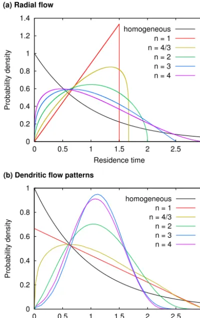
Figure 4 shows the residence time distributions of the ex-amples considered in Sects. 4.1 and 4.2, obtained by evaluat-ing the path integrals over v(1x)according to Eq. (49) numer-ically. Both geometries yield exponential residence time dis-tributions for a homogeneous aquifer, but completely differ-ent distributions otherwise. In the example of radial flow, the distribution changes from being strongly negatively skewed to positively skewed for increasingn. The respective distribu-tions of the dendritic networks are always positively skewed and become more symmetric for increasingn. Forn=2 or not much larger, which was found to be the most reasonable range, the distributions are moderately positively skewed in both examples.
The residence time distribution for radial flow can be ex-plained directly with Eq. (50) since the flow rate is entirely determined by the recharge and thus independent ofn, the same as for a homogeneous aquifer. For small values ofn, the increase in velocity towards the spring is much weaker than in the homogeneous case. As this affects the residence times in the entire catchment, it results in high residence times for large parts of the catchment. In return, the velocities approach those of the homogeneous distribution forn→ ∞, resulting in a positively skewed residence time distribution.
(b) Dendritic flow patterns
0 0.2 0.4 0.6 0.8 1
0 0.5 1 1.5 2 2.5 3
Probability density
Residence time homogeneous
n = 1 n = 4/3 n = 2 n = 3 n = 4 (a) Radial flow
0 0.2 0.4 0.6 0.8 1 1.2 1.4
0 0.5 1 1.5 2 2.5 3
Probability density
Residence time homogeneous
[image:9.612.67.268.67.387.2]n = 1 n = 4/3 n = 2 n = 3 n = 4
Figure 4. Residence time distributions for the two examples consid-ered in Sects. 4.1 (a) and 4.2 (b). The nondimensional time axis is scaled in such a way that the mean residence time is one for the ho-mogeneous distribution of the conductivity, and the total pore space volume is the same in all cases.
the dependence on nis rather weak. Notably, the residence time distributions obtained forn≥2 are similar to those aris-ing from an advection–dispersion model, although the theory behind our model is completely different from this.
5 Extension towards turbulent flow
The theory presented in this paper hinges on laminar flow according to Darcy’s law, while flow becomes turbulent at large flow rates in reality. This particularly applies to large conduits in karstic systems. In the following we give a sketch of an extension of our theory towards turbulent flow.
Let us first assume fully turbulent flow through parallel conduits of radiiri, so that the flow in each of them is de-scribed by the Darcy–Weisbach law:
|∇h(x)| ∝v
2 i
ri , (51)
with the flow velocityvi. Then the volumetric flow rate is
q(x)∝X
i
ri2vi∝
p
|∇h(x)|X
i
ri2√ri, (52)
which can also be written as
|∇h(x)| ∝ q(x)
2
P
i r
5 2
i
2. (53)
If we increase all radii by the same factorβ, the denominator increases by a factorβ5, corresponding toφ52. In analogy to
the laminar case (Eq. 17) we can alternatively assume that the only largest conduit is widened and obtain
∂log|∇h|
∂logφ = φ
|∇h|
∂|∇h|
∂φ = φ
|∇h|
∂|∇h|
∂rmax
∂φ ∂rmax
= −5
2
P
i
ri2√rmax
P
i r
5 2
i
≤ −5
2. (54)
We therefore assume
|∇h(x)| ∝ q(x)
2
φ (x)m, (55)
withm≥5
2. Inserting this approach into Eq. (6) yields P ∝
Z q(x)3 φ (x)md
3x. (56)
Minimizing this expression under the constraint of a given total pore space volume (Eq. 11) requires
∂P
∂φ (x)= −m q(x)3
φ (x)m+1=constant, (57) and thus
φ (x)∝q(x)m3+1. (58)
This increase of the optimal porosity with the volumetric flow rate is even stronger than the increase likeqn+21 with
n≥2 found for laminar flow (Eq. 24). Inserting the re-spective version of Eq. (24) with m3+1 instead of n+21 into Eq. (56) leads to
P ∝ Z
q(x)m3+1d3x
m+1
, (59)
so that the functional to be minimized is G(q)=
Z
q(x)m3+1d3x. (60)
for all valuesm≥5
2, but closer to one than the exponent 2 n+1 for laminar flow. The lowest value,m=5
2, is equivalent to the laminar case forn=4
3(which is unrealistic for laminar flow as we foundn≥2 there). Repeating the calculations leading to Eq. (50) for turbulent flow reveals that the same result also holds for the residence time distributions.
Due to this equivalence, the upper left network shown in Fig. 1 (n=4
3, equivalent tom= 5
2) illustrates that fully turbu-lent flow conditions result in less dendritic flow patterns than laminar flow conditions. But, as shown in Fig. 2, the size dis-tribution of the spring discharges is not affected. However, the residence time distribution (Fig. 4b) becomes strongly skewed in the turbulent regime. So some of the properties of the flow network are basically the same for laminar and tur-bulent flow, while some other properties change significantly. However, the most significant effect of turbulence should occur at the transition from laminar to turbulent flow. This transition is in general accompanied by a strong increase in energy dissipation. For an individual pipe, the transition oc-curs when the Reynolds number exceeds a given threshold. The Reynolds number itself is proportional to the radius of the pipe and to the flow velocity. In our approach, the radii increase with the porosity and thus with the discharge. Ac-cording to Eq. (50), the flow velocity also increases with the discharge, so that the Reynolds number increases with the discharge, too. As a consequence, the transition to turbulent flow shall occur at a given critical flow rate. This also implies that the turbulent regime can only cover a part of the domain in general. Therefore, the functional to be minimized will be-come more complicated than the one given in Eq. (4): G(q)=
Z
f (q(x))q(x)γ (q(x))d3x, (61) or for discrete networks
G(q)=X
i
f (qi) qγ (qi)
i , (62)
wheref (q)=1 andγ (q)= 2
n+1 ifq is below the turbulent threshold, while f (q)=constant>1 andγ (q)= 3
m+1 else. As this functional is even discontinuous, the minimization becomes nontrivial, and it is not even clear whether the con-jecture that each site has a unique flow direction holds in the region close to the transition.
6 Limitations
Although our first results are promising, some limitations of the new theory are already visible. While the theory in itself should be consistent, these limitations concern the relevance of the thermodynamic limit of minimum energy dissipation for real subsurface flow patterns.
Even if we assume that the evolution of porosity goes in direction of minimizing energy dissipation, the question
remains whether a self-organizing porosity distribution start-ing from a given state is really able to come close to the ground state of minimum energy dissipation. In karst systems where the evolution of porosity due to solution is understood quite well at small scales, this evolution is always directed towards higher porosity. Even if we assume that any increase in porosity is spent in such a way that the energy dissipation is reduced most efficiently, more or less parallel preferen-tial flow paths may arise first even at rather small distances. Removing one of them in order to obtain a more dendritic and thus energetically better network may require a strong further increase in porosity which may be impossible in real-ity. Therefore, the spatial scale up to which the optimization can proceed may be limited in reality and so far there has not been a quantitative relationship between this scale and the to-tal (increase in) porosity. At first sight this seems to be a strik-ing difference towards the evolution of river networks at the surface. Due to erosion and uplift permanently counteracting each other, a river network may in principle have unlimited time to self-organize. However, as shown by Hergarten and Neugebauer (2001), the ability of river networks to erase ex-isting patterns is also limited, so that the problem is basically the same as for subsurface flow. And as pointed out before, the considered statistical properties of both subsurface and surface flow networks are not very helpful in this context as they are rather insensitive to the distance from the ground state of minimum energy dissipation.
As a second major aspect, the examples presented in Sect. 4 are horizontal two-dimensional flow patterns and do not include a vertical component. For three-dimensional flow patterns, the recharge applied to the entire domain in two di-mensions must be replaced by an influx at the upper bound-ary. It is easily recognized that the optimal flow pattern then starts with horizontal flow along the upper boundary keeping the lower regions dry as this is the fastest way to focus flow. If the level where water leaves the domain at the sides is lower, the preferential flow paths will approach this lower level only close to the side boundaries. In reality, there is a tendency to-wards vertical flow from the beginning, which means that the idea of minimum energy dissipation can only work in three dimensions if the anisotropy due to gravity is incorporated in an appropriate way. Such an extension should include a re-duced energy dissipation for vertical flow, but its quantitative representation is not yet clear.
7 Conclusions
more complicated. Beyond the basic equations, we have to introduce different constraints for the minimization. While equilibrium between tectonic uplift and erosion is assumed for river networks, we assume a given total pore space vol-ume and a relationship between porosity and permeability.
Despite the differences in the theories, both concepts fi-nally arrive at basically the same functional to be minimized. As a consequence, the predicted preferential flow patterns in two dimensions are quite similar to surface river networks. The predicted size distribution of the spring discharges fol-lows a power law with a (noncumulative) scaling exponent τ=1.5. This result reproduces the spring size distributions of two regions in Austria quite well, although the scaling ex-ponent seems to be slightly higher there, namelyτ≈1.8. The other application shown in this paper, radial flow towards a spring, suggests how the transmissivities in the region around a spring might be chosen in a model where preferential flow patterns are not taken into account explicitly.
The residence time distributions seem to be the most strik-ing difference between our model for subsurface flow and rivers at the surface. In contrast to rivers, our theory predicts an increase of flow velocity with flow rate, which is, how-ever, not as strong as in an homogeneous aquifer. As a con-sequence of the weaker increase, mean residence times are in general higher for optimized flow patterns than for homoge-neous aquifers.
Finally, it should not be forgotten that, similarly to all other principles of optimization in hydrology, the question remains whether real systems indeed organize towards their thermo-dynamic limit and, if so, how close can they come to the op-timized state. The validation based on spring discharge dis-tributions is promising, but does not prove that flow patterns indeed self-organize according to minimum energy dissipa-tion. Therefore, further studies are needed in order to inves-tigate the applicability of our hypothesis. These studies will also have to include three-dimensional flow patterns and the influence of external predesign.
Acknowledgements. This work was funded by the Austrian Science Fund (FWF): L576-N21, the European Regional Development Fund (ERDF), and the Federal Government of Styria. Spring discharge data of the Semmering region were provided by the Austrian Federal Railways ÖBB Infrastruktur AG. The help of M. Westhoff and A. Kleidon in improving the clarity of the manuscript is greatly appreciated.
Edited by: M. Weiler
References
Banavar, J. R., Maritan, A., and Rinaldo, A.: Size and form in efficient transportation networks, Nature, 399, 130–132, doi:10.1038/20144, 1999.
Birk, S. and Hergarten, S.: Estimation of aquifer parameters from the recession of spring hydrographs – Influence of flow geometry, Geophys. Res. Abstr., 14, EGU2012-9777, 2012.
Carman, P. C.: Fluid flow through granular beds, Trans. Inst. Chem. Engin. London, 15, 150–166, 1937.
Dreybrodt, W., Gabrovšek, F., and Romanov, D.: Processes of Speleogenesis: a Modeling Approach, vol. 4 of Carsologica, ZRC Publishing, Ljubljana, 2005.
Enquist, B. J., Brown, J. H., and West, G. B.: Allometric scaling of plant energetics and population density, Nature, 395, 163–165, doi:10.1038/25977, 1998.
Enquist, B. J., West, G. B., Charnov, E. L., and Brown, J. H.: Allo-metric scaling of production and life-history variation in vascular plants, Nature, 401, 907–911, doi:10.1038/44819, 1999. Gabrovšek, F. and Dreybrodt, W.: Spreading of tracer plumes
through confined telogenetic karst aquifers: a model, J. Hydrol., 409, 20–29, doi:10.1016/j.jhydrol.2011.07.029, 2011.
Groves, C. G. and Howard, A. D.: Early development of karst sys-tems: 1. Preferential flow path enlargement under laminar flow, Water Resour. Res., 30, 2837–2846, doi:10.1029/94WR01303, 1994.
Hack, J. T.: Studies of longitudinal profiles in Virginia and Mary-land, no. 294-B in US Geol. Survey Prof. Papers, US Govern-ment Printing Office, Washington, D.C., 1957.
Hergarten, S.: Self-Organized Criticality in Earth Systems, Springer, Berlin, Heidelberg, New York, 2002.
Hergarten, S. and Neugebauer, H. J.: Self-organized criti-cal drainage networks, Phys. Rev. Lett., 86, 2689–2692, doi:10.1103/PhysRevLett.86.2689, 2001.
Horton, R. E.: Erosional development of streams and their drainage basins; hydrophysical approach to quantitative morphology, Bull. Geol. Soc. Am., 56, 275–370, 1945.
Howard, A. D.: Theoretical model of optimal drainage networks, Water Resour. Res., 26, 2107–2117, doi:10.1029/WR026i009p02107, 1990.
Howard, A. D.: A detachment-limited model for drainage basin evo-lution, Water Resour. Res., 30, 2261–2285, 1994.
Howard, A. D. and Groves, C. G.: Early development of karst systems: 2. Turbulent flow, Water Resour. Res., 31, 19–26, doi:10.1029/94WR01964, 1995.
Hubinger, B. and Birk, S.: Influence of initial heterogeneities and recharge limitations on the evolution of aperture distributions in carbonate aquifers, Hydrol. Earth Syst. Sci., 15, 3715–3729, doi:10.5194/hess-15-3715-2011, 2011.
Kaufmann, G. and Braun, J.: Karst aquifer evolution in fractured rocks, Water Resour. Res., 35, 3223–3238, doi:10.1029/1999WR900169, 1999.
Kaufmann, G. and Braun, J.: Karst aquifer evolution in frac-tured, porous rocks, Water Resour. Res., 36, 1381–1391, doi:10.1029/1999WR900356, 2000.
Kiraly, L.: Remarques sur le simulation des failles et du réseau kars-tique par élèments finis dans les modelès d’ècoulement, Bull. Centre Hydrogéol., 3, 155–167, 1979.
Kleidon, A. and Renner, M.: Thermodynamic limits of hydrologic cycling within the Earth system: concepts, estimates and implica-tions, Hydrol. Earth Syst. Sci., 17, 2873–2892, doi:10.5194/hess-17-2873-2013, 2013.
Kleidon, A. and Schymanski, S. J.: Thermodynamics and optimality of the water budget on land: a review, Geophys. Res. Lett., 35, L20404, doi:10.1029/2008GL035393, 2008.
Kleidon, A., Zehe, E., Ehret, U., and Scherer, U.: Thermodynam-ics, maximum power, and the dynamics of preferential river flow structures at the continental scale, Hydrol. Earth Syst. Sci., 17, 225–251, doi:10.5194/hess-17-225-2013, 2013.
Kleidon, A., Renner, M., and Porada, P.: Estimates of the climato-logical land surface energy and water balance derived from maxi-mum convective power, Hydrol. Earth Syst. Sci., 18, 2201–2218, doi:10.5194/hess-18-2201-2014, 2014.
Kozeny, J.: Über kapillare Leitung des Wassers im Boden, Sitzungs-ber. Akad. Wiss. Wien, 136, 271–306, 1927.
Liedl, R., Sauter, M., Hückinghaus, D., Clemens, T., and Teutsch, G.: Simulation of the development of karst aquifers using a cou-pled continuum pipe flow model, Water Resour. Res., 39, 1057, doi:10.1029/2001WR001206, 2003.
Martyushev, L. M.: Entropy and entropy production: old mis-conceptions and new breakthroughs, Entropy, 15, 1152–1170, doi:10.3390/e15041152, 2013.
McDonnell, J. J., Sivapalan, M., Vaché, K., Dunn, S., Grant, G., Haggerty, R., Hinz, C., Hooper, R., Kirchner, J., Roderick, M. L., Selker, J., and Weiler, M.: Moving beyond heterogeneity and pro-cess complexity: a new vision for watershed hydrology, Water Resour. Res., 42, W07301, doi:10.1029/2006WR005467, 2007. Metropolis, N., Rosenbluth, A. W., Rosenbluth, M. N., Teller,
A. H., and Teller, E.: Equation of state calculations by fast computing machines, J. Chem. Phys., 21, 1087–1092, doi:10.1063/1.1699114, 1953.
Rinaldo, A., Rodriguez-Iturbe, I., Bras, R. L., Ijjasz-Vasquez, E., and Marani, A.: Minimum energy and fractal structures of drainage networks, Water Resour. Res., 28, 2181–2195, 1992. Rinaldo, A., Rodriguez-Iturbe, I., and Rigon, R.: Channel
networks, Annu. Rev. Earth Planet. Sci., 26, 289–327, doi:10.1146/annurev.earth.26.1.289, 1998.
Rodriguez-Iturbe, I., Rinaldo, A., Rigon, R., Bras, R. L., Ijjasz-Vasquez, E., and Marani, A.: Fractal structures as least energy patterns: The case of river networks, Geophys. Res. Lett., 19, 889–892, doi:10.1029/92GL00938, 1992a.
Rodriguez-Iturbe, I., Rinaldo, A., Rigon, R., Bras, R. L., Marani, A., and Ijjasz-Vasquez, E.: Energy dissipation, runoff production, and the three-dimensional structure of river basins, Water Resour. Res., 28, 1095–1103, doi:10.1029/91WR03034, 1992b. Siemers, J. and Dreybrodt, W.: Early development of Karst aquifers
on percolation networks of fractures in limestone, Water Resour. Res., 34, 409–419, doi:10.1029/97WR03218, 1998.
West, G. B., Brown, J. H., and Enquist, B. J.: A general model for the origin of allometric scaling laws in biology, Science, 276, 122–126, doi:10.1126/science.276.5309.122, 1997.
West, G. B., Brown, J. H., and Enquist, B. J.: A general model for the structure and allometry of plant vascular systems, Nature, 400, 664–667, doi:10.1038/23251, 1999a.
West, G. B., Brown, J. H., and Enquist, B. J.: The fourth dimen-sion of life: fractal geometry and allometric scaling of organisms, Science, 284, 1677–1679, doi:10.1126/science.284.5420.1677, 1999b.
Westhoff, M. C. and Zehe, E.: Maximum entropy production: can it be used to constrain conceptual hydrological models?, Hy-drol. Earth Syst. Sci., 17, 3141–3157, doi:10.5194/hess-17-3141-2013, 2013.
Zehe, E., Blume, T., and Blöschl, G.: The principle of maximum energy dissipation: a novel thermodynamic perspective on rapid water flow in connected soil structures, Philos. T. Roy. Soc. B, 365, 1377–1386, doi:10.1098/rstb.2009.0308, 2010.
Zehe, E., Ehret, U., Blume, T., Kleidon, A., Scherer, U., and West-hoff, M.: A thermodynamic approach to link self-organization, preferential flow and rainfall–runoff behaviour, Hydrol. Earth Syst. Sci., 17, 4297–4322, doi:10.5194/hess-17-4297-2013, 2013.