A physically based approach for the estimation of root zone soil moisture from surface measurements

www.hydrol-earth-syst-sci.net/18/1199/2014/ doi:10.5194/hess-18-1199-2014

© Author(s) 2014. CC Attribution 3.0 License.

Hydrology and

Earth System

Sciences

A physically based approach for the estimation of root-zone soil

moisture from surface measurements

S. Manfreda1, L. Brocca2, T. Moramarco2, F. Melone2, and J. Sheffield3 1_{School of Engineering, University of Basilicata, Potenza, Italy}

2_{Research Institute for Geo-Hydrological Protection (IRPI), National Research Council, Perugia, Italy} 3_{Department of Civil and Environmental Engineering, Princeton University, Princeton, NJ, USA}

Correspondence to: S. Manfreda ([email protected])

Received: 3 October 2012 – Published in Hydrol. Earth Syst. Sci. Discuss.: 20 December 2012 Revised: 27 January 2014 – Accepted: 10 February 2014 – Published: 28 March 2014

Abstract. In the present work, we developed a new

formu-lation for the estimation of the soil moisture in the root zone based on the measured value of soil moisture at the surface. It was derived from a simplified soil water balance equa-tion for semiarid environments that provides a closed form of the relationship between the root zone and the surface soil moisture with a limited number of physically consistent parameters. The method sheds lights on the mentioned re-lationship with possible applications in the use of satellite remote sensing retrievals of soil moisture. The proposed ap-proach was used on soil moisture measurements taken from the African Monsoon Multidisciplinary Analysis (AMMA) and the Soil Climate Analysis Network (SCAN) databases. The AMMA network was designed with the aim to mon-itor three so-called mesoscale sites (super sites) located in Benin, Mali, and Niger using point measurements at differ-ent locations. Thereafter the new formulation was tested on three additional stations of SCAN in the state of New Mex-ico (US). Both databases are ideal for the application of such method, because they provide a good description of the soil moisture dynamics at the surface and the root zone using probes installed at different depths. The model was first ap-plied with parameters assigned based on the physical char-acteristics of several sites. These results highlighted the po-tential of the methodology, providing a good description of the root-zone soil moisture. In the second part of the paper, the model performances were compared with those of the well-known exponential filter. Results show that this new ap-proach provides good performances after calibration with a set of parameters consistent with the physical characteristics

of the investigated areas. The limited number of parameters and their physical interpretation makes the procedure appeal-ing for further applications to other regions.

1 Introduction

An important contribution was given by Wagner et al. (1999), who suggested the use of an exponential filter of the form exp(−t /T ), whereT is the characteristic length time or recession constant. This filter was used to convert the time series of surface measurements to a signal that is able to capture the dynamics of the lower soil layer. The great ad-vantage of this filter lies in its simplicity due to the fact that it makes use of one parameter only. Moreover, the derived soil moisture index (SWI) relies only on the surface observation (remotely sensed data). Therefore, this approach, which from now on will be referred to as the SWI method, has been tested with both simulated and measured data, providing good re-sults, and has been extensively used to improve the descrip-tion of the root-zone soil moisture in rainfall–runoff applica-tions (e.g. Manfreda et al., 2011; Brocca et al., 2010, 2012; Matgen et al., 2012a).

The growing interest in this approach makes it critical to provide a physical interpretation of the parameterT that is influenced by a number of physical processes controlling soil moisture fluctuations. Several authors have tackled this problem (e.g. Ceballos et al., 2005; De Lange et al., 2008; Albergel et al., 2008). For instance, Ceballos et al. (2005) demonstrated thatT represents the parameter of the exponen-tial autocorrelation function of soil moisture. For this reason, T is influenced by all the physical processes affecting the temporal fluctuations of soil moisture (e.g. evapotranspira-tion, soil hydraulic properties, soil depth, number of soil lay-ers, etc.). In this way, they demonstrated that the parameterT is proportional to the ratio between the soil water content at field capacity and potential evapotranspiration. De Lange et al. (2008) tested the model for several soil textures using sim-ulated data obtained with the finite-element HYDRUS-1D model. They demonstrated the strong influence that the soil parameters and the sampling periods have onT. According to these findings, the authors suggested that the SWI method-ology should benefit from a soil texture differentiation. An-other attempt to give a physical interpretation of the reces-sion constant (T) was carried out by Albergel et al. (2008), who investigated the correlation of the parameter,T, with soil properties and climate conditions over France. Unfortu-nately, they did not observe significant relationships between T and the main soil properties (clay and sand fractions, bulk density and organic matter content).

An alternative and increasingly more useful approach is to assimilate satellite retrievals into land surface models (e.g. Reichle et al., 2002, 2004). Such an approach has benefitted from the progress made in recent years on assimilation meth-ods and the availability of long-term records of retrievals from either microwave (e.g. Scipal et al., 2008) or thermal sensors (e.g. Crow et al., 2008), or both (e.g. Li et al., 2010). The purpose of this paper is not to define an operational approach in place of assimilation systems, but to shed light on a phenomenon of general interest. The approach proposed here represents an attempt to describe analytically the rela-tionship between the surface soil moisture and the root-zone

soil moisture value using parameters that are related to the physical characteristics of the site under investigation. In this way, one may infer the soil moisture state below the surface using surface soil moisture data along with some physical characteristics of the site. The model presented herein repre-sents an attempt to tackle this problem, providing a solution that may be considered reliable in dry areas. Our preliminary application has been carried out using soil moisture obser-vations taken from the African Monsoon Multidisciplinary Analysis (AMMA) and the Soil Climate Analysis Network (SCAN) databases. These two networks represent valuable sources of soil moisture data measured at different depths that is shared via the web with the entire scientific commu-nity. In this way, these data have been involved in a signif-icant number of calibration and validation activities that in-creases the interest and the information contents related to these networks. For the scope of this paper, we selected a number of stations with detailed information along the soil profile and also with some information on the soil texture. All stations have been selected in arid and semiarid environ-ments. The results obtained are extremely encouraging and the methodology may represent a useful tool under some spe-cific climatic conditions.

The paper is organized with a presentation of the new model in Sect. 2, where the SWI method is also described. Section 3 provides a description of the AMMA and SCAN databases and, finally, in Sect. 4, which precedes the conclu-sion, the model is applied for the AMMA and SCAN data and its performances are compared with those of the SWI method.

2 Model description

2.1 Soil moisture analytical relationship (SMAR)

Several hydrological models are based on a conceptual scheme with multiple layers in order to describe the soil moisture profile. Models that make use of remotely sensed data in assimilation frequently use such a representation with a surface layer of a few centimetres (e.g. Brocca et al., 2012). In the present work, the soil is assumed to be composed of two layers, one at the surface with a depth of a few centime-tres (equivalent to the retrieval depth of the satellite sensor) and a second one below with a depth that may be assumed coincident with the rooting depth of vegetation (of the order of 60–150 cm). From here on, we will refer to those as the first and second layer, respectively, and we will use a sub-script “1” or “2” to distinguish between their variables and parameters.

as a function of rainfall, but of the soil moisture content in the surface soil layer. This may allow the derivation of a function of the soil moisture in one layer as a function of the other one. The water flux from the top layer can be considered sig-nificant only when the soil moisture exceeds field capacity. Assuming that the soil moisture movement from the upper to the lower layer during a rainfall event can be modelled fol-lowing the Green–Ampt approach (Green and Ampt, 1911), one can assume that all water in the first layer above field capacity will move into the lower layer within one day. This idea was inspired by the work of Laio (2006), who proposed a model for the description of the soil moisture profile.

Under such assumptions, the infiltration flux from the top layer to the lower occurs instantaneously and is described by

n1Zr1y(t )=n1Zr1y[s1(t ), t]

=n1Zr1

(s1(t )−sc1) , s1(t )≥sc1

0, s1(t ) < sc1, (1)

wherey(t )[–] fraction of soil saturation infiltrating in the lower layer,n1[–] is the soil porosity of the first layer, Zr1

[L] is the depth of the first layer,s1(θ1/n1) [–] is the relative

saturation of the first layer (given by the ratio between the soil water content,θ1, and the porosity,n1, of the first layer),

andsc1[–] is the value of relative saturation at field capacity

of the first layer of soil.

The above equation implies the assumption of an infinite permeability of the soil when the relative saturation reaches any value above field capacity. It is also necessary that the first layer not be infinitesimal, because this condition will lead to zero infiltration. Moreover, the model does not ac-count for the saturation effect of the lower layer. It is neces-sary to note that, in order to avoid undesired underestimation of the infiltration, the surface soil moisture value should be referred to the first 5–10 cm of soil. A thickness of less than 5 cm may lead to numerical problems in this and other hydro-logical models. For this reason, several hydrohydro-logical mod-els that incorporate a surface layer in the soil description, assume a thickness of about 10 cm (e.g. Liang et al., 1994, 1996; Wood et al., 1997). Most satellite sensors cannot pen-etrate deeper than a few centimetres, but it is a reasonable assumption that these measures can be representative of the dynamics of a surface layer of approximately 5–10 cm.

Following this reasoning, the soil water balance of the second and deeper soil layer is controlled by two main fac-tors: infiltration and soil water losses. Given the infiltration equation, we can continue with a simplified approach assum-ing a linear soil water loss function that includes both evap-otranspiration and percolation (e.g. Porporato et al., 2004; Rodriguez-Iturbe et al., 2006). Both these processes are neg-ligible when the soil saturation is below the wilting point. For this reason we assumed that the soil losses decrease linearly from a maximum value under well-watered conditions to 0 at the wilting point.

Definingx2=(s2−sw2) / (1−sw2)as the “effective”

rel-ative soil saturation of the second soil layer and w0=

(1−sw2) n2Zr2the soil water storage, the soil water balance

can be described by the following expression: (1−sw2) n2Zr2

dx2(t )

dt =n1Zr1y(t )−V2x2(t ), (2) wheres2[–] represents the relative saturation of the soil,sw2

[–] is the relative saturation at the wilting point,n2[–] is the

soil porosity, Zr2[L] is the soil depth,V2[L T−1] is the soil

water loss coefficient accounting for both evapotranspiration and percolation losses, andx2 [–] is the “effective” relative

soil saturation of the second soil layer.

It should be noted that this equation does not account for the high non-linearity that characterizes the soil loss function for high values of soil moisture. This simplification, along with the fact that the infiltration does not account for the sat-uration effect, implies some limitations in the use of such an approach in humid environments. The model in fact was thought mainly for a semiarid environments with flat surfaces and neglecting the presence of phreatic surfaces, effects due to topographic convergence (e.g. subsurface flows), the pres-ence of frozen soils, etc.

The equation above can be simplified using normalized co-efficientsaandbdefined as

a= V2

(1−sw2) n2Zr2

, b= n1Zr1 (1−sw2) n2Zr2

. (3)

The value of these parameters can be related directly to the ratio of the depths of the two layers and the soil water loss co-efficient. As a consequence, the soil water balance equation becomes

dx2(t )

dt =b y(t )−a x2(t ). (4)

It is interesting to note that this equation represents a gen-eralization that also includes the case proposed by Wagner et al. (1999). Assuming an initial condition for the relative saturationx2(t )equal to zero, one may derive an analytical

solution to this linear differential equation:

x2(t )= t

Z

0

b ea(w−t )y(w)dw . (5)

For practical applications, one may need the discrete form as well:

x2(tj)= j

X

i=0

b ea(ti−tj)y(t

i)1t . (6)

Expanding Eq. (6) and assuming1t= tj−t(j−1), one

may derive the following expression for the soil moisture in the second layer based on the time series of surface soil mois-ture:

that may be rewritten as a function ofs2as

s2(tj)=sw2+ s2 tj−1−sw2e−a(tj−tj−1)

+(1−sw2) b y tj tj−tj−1. (8)

The method proposed here represents a soil moisture an-alytical relationship (from now on we will refer to it as SMAR) between the two state variables introduced with the four parameterssw2,sc1,a, andb. All these parameters may

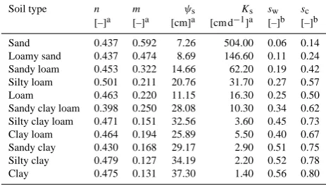
be estimated from the soil texture, the soil depth, and the soil water losses. The parameterais a function of potential evap-otranspiration and soil permeability that can be estimated us-ing regression functions such as those proposed by Pan et al. (2003). It should be noted that SMAR may produce values higher than 1 and that these are automatically set equal to 1. In order to provide a range of variability of the soil pa-rameters of the model, Table 1 collects the values derived from the experimental investigations by Rawls and Brak-ensiek (1989) and also reported in Rawls et al. (1993). In particular, the soil porosity (n), the bubbling pressure head (ψ), and the soil permeability at saturation (Ks) were taken

from Rawls et al. (1993), while the values ofswandschave

been calculated adopting the Brooks and Corey (1964) model (ψ (s)=ψss−1/m, wheremis the pore-size index) assuming

a soil water potential ofψ= −1.5 Mpa and−0.03 Mpa, re-spectively.

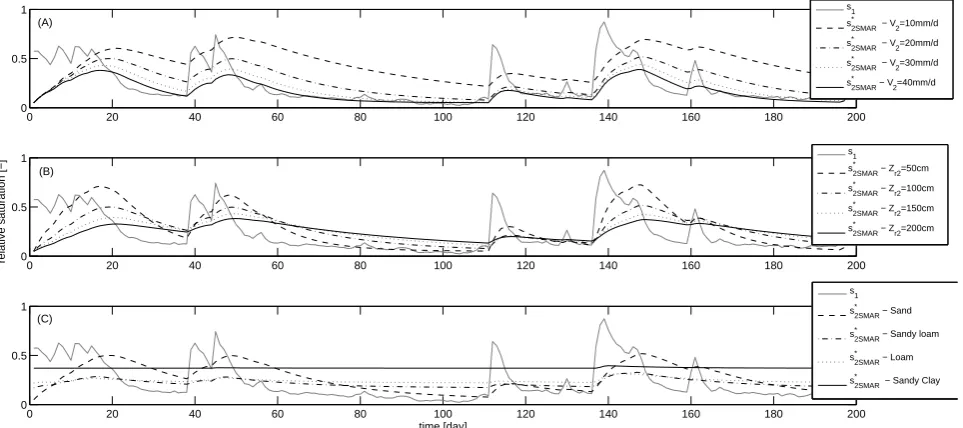
Figure 1 shows some examples of the application of SMAR in a short time series of surface soil moisture mea-sured in the first 10 cm of soil in a dry environment (mea-surements are taken from the station of Sevilleta, New Mex-ico, US). This preliminary application is used to show the in-fluence that different model parameters have on the derived root-zone soil moisture, nameds_2SMAR∗ . With this specific aim, we plotted the derived soil moisture in the root zone as-suming a different combination of parameters changing the values of the soil water loss coefficient (Fig. 1a); the depth of the second soil layer (Fig. 1b); and the soil parameters as-sociated with different soil textures (Fig. 1c). The function s∗_2SMARis obtained via changing the parametersV2and Zr2

in Fig. 1a and b, respectively, while the functions plotted in Fig. 1c are obtained assuming different soil textures using the values reported in Table 1. In each plot, the remaining parameters have been assumed constant using as reference values the following set of parameters: n1=n2=0.437,

sw2=0.06, sc2=0.14, V =2 cm day−1, Zr1=10 cm, and

Zr2=100 cm. Alls_2SMAR∗ time series have been computed

assigning the relative saturation at field capacity as the ini-tial value. All functions have been plotted assuming as iniini-tial value for the soil moisture in the second soil layer equal to the field capacity.

This preliminary analysis was useful to understand the role of each parameter for the soil moisture dynamics. In particu-lar, the water loss coefficient produces a shift on the function s∗_2SMAR, preserving the general pattern with a reduction of the mean value of the soil moisture with the increase ofV2.

Table 1. Soil parameters associated with different soil textures

ac-cording to the experiments by Rawls and Brakensiek (1989).a Pa-rameters taken from Rawls and Brakensiek (1989) and also reported in Rawls et al. (1993).bThe relative saturation at the wilting point and the field capacity have been estimated using the Brooks–Corey model assumingψ= −1.5 and−0.03 Mpa, respectively.

Soil type n m ψs Ks sw sc

[–]a [–]a [cm]a [cm d−1]a [–]b [–]b

Sand 0.437 0.592 7.26 504.00 0.06 0.14

Loamy sand 0.437 0.474 8.69 146.60 0.11 0.24

Sandy loam 0.453 0.322 14.66 62.20 0.19 0.42

Silty loam 0.501 0.211 20.76 31.70 0.27 0.57

Loam 0.463 0.220 11.15 16.30 0.25 0.50

Sandy clay loam 0.398 0.250 28.08 10.30 0.34 0.62

Silty clay loam 0.471 0.151 32.56 3.60 0.45 0.73

Clay loam 0.464 0.194 25.89 5.50 0.40 0.67

Sandy clay 0.430 0.168 29.17 2.90 0.51 0.75

Silty clay 0.479 0.127 34.19 2.20 0.52 0.78

Clay 0.475 0.131 37.30 1.40 0.56 0.80

The impact of the depth of the second layer of soil produces a significant modification on the variability of the soil moisture that increases with the reduction of the Zr2 values. Finally,

the soil texture also has a critical role, affecting several model parameters. In the present scheme, it was assumed that the soil texture controls the values of soil porosity, the relative saturation at the field capacity and at the wilting point. These last two parameters impact on the minimum value reached by thes_2SMAR∗ and the variability of the soil moisture. In par-ticular, the fluctuations of soil moisture increase for lower values ofsc1. In fact, we observed a continuous reduction in

the fluctuations moving from sand to sandy clay soil. In this last case, the value ofsc1is so high that it inhibits most of the

infiltration in the lower soil layer, and as a consequence soil moisture remains almost constant around the value of wilting point. It is necessary to point out that different soil textures have also different permeability, which may affect the value of the soil water loss coefficient, which in the present case was kept constant.

At this point, the comparison between the proposed pro-cedure and the SWI method becomes extremely interesting, and will be described better and in greater detail in the fol-lowing section.

2.2 Exponential filter

0 20 40 60 80 100 120 140 160 180 200 0

0.5 1

(A)

s₁ s

2 *

SMAR − V2=10mm/d

s₂*_SMAR − V₂=20mm/d s₂*_SMAR − V₂=30mm/d s₂*_SMAR − V₂=40mm/d

0 20 40 60 80 100 120 140 160 180 200

0 0.5 1

relative saturation [−]

(B)

s

1

s₂*_SMAR − Z_r2=50cm s₂*_SMAR − Z_r2=100cm s₂*_SMAR − Z_r2=150cm s₂*_SMAR − Z_r2=200cm

0 20 40 60 80 100 120 140 160 180 200

0 0.5 1

time [day] (C)

s₁ s₂*_SMAR − Sand s

2 *

SMAR − Sandy loam

s₂*_SMAR − Loam s

2 *

SMAR − Sandy Clay

Fig. 1. Examples of application of the SMAR to a time series of surface soil moisture (s1, relative saturation of the first 10 cm of soil) for

different values of soil water losses (A), rooting depth ratios (B), and soil textures (C). The functions_2SMAR∗ is obtained through changing only one parameter in (A) and (B) (V and Zr₂, respectively) and assigning different soil textures in (C) using the soil parameters reported in Table 1. In each plot, the remaining parameters have been assigned using the following set of reference valuesn1=n2=0.437,sw2=0.06,

sc2=0.14,V=2 cm day−1, Zr1=10 cm, and Zr2=90 cm (measurements are taken from the station of Sevilleta – lat. 34◦210N, long.

106◦410W; New Mexico, US).

change existing between the surface soil moisture and the deeper soil layer.

Following the same notation as has been used above, the soil water balance equation may be written as

nZrds2

dt =C (s1−s2) , (9)

wheret is the time andC is a pseudodiffusivity coefficient that depends on the soil properties. This method assumes that the variation of the root-zone soil moisture is linearly related to the difference between the surface and root-zone soil mois-ture. One may immediately realize that the equation contains only one parameter that is represented byT =nZr/C, named the characteristic time length.

This approach leads to the development of an exponential filter that has been extensively used in remote sensing appli-cations, but with the limitation of a physical interpretation of the parameterT. The root-zone soil moisture can be obtained through the knowledge of the surface soil moisture and a pa-rameterT. The recursive formulation of the method relies on (Albergel et al., 2008)

s∗₂ tj

=s₂∗ tj−1+Kj

s1 tj

−s₂∗ tj−1, (10)

wheres₂∗ tj

is the soil moisture of the second layer esti-mated through the exponential filter (usually defined as the soil water index). The gainKj at timetjis given by (in a

re-cursive form)

Kj=

Kj−1

Kj−1+e

−tj−tj−1 T

(11)

and it ranges between 0 and 1. For the initialization of this filter,K1ands₂∗(t1)were set to 1 ands2(t1), respectively.

3 Data description: in situ observations

3.1 The AMMA database

The proposed method (SMAR) was tested using field mea-surements at various depths of three sites of the AMMA database. The AMMA database user interface for accessing local and satellite data is found at AMMA Database (2014). These and other soil moisture products from other projects have been collected in the International Soil Moisture Net-work (ISMN) database1(e.g. Dorigo et al., 2011). The data set presented in this paragraph was downloaded from the ISMN database.

The AMMA programme is an international long-term col-laboration to study the climatic and environmental feedback mechanisms involved in the African monsoon, and in some of its consequences on society and human health. The pro-gramme, which started in 2004, has developed a network

of ground-based observation stations over sub-Saharan West Africa, and several intensive measurement campaigns (see Redelsperger et al., 2006). In particular, three mesoscale sites were implemented in Benin (Pellarin et al., 2009b), Mali (de Rosnay et al., 2009), and Niger (Pellarin et al., 2009a), pro-viding a large amount of information on soil moisture and many other variables. In the present paper, we focused on the point measurements taken at the sites of Nalohou-Mid and Nalohou-Top in Benin, Agoufou in Mali, and Wankama and Tondikiboro in Niger. The climate conditions of these three sites are significantly different in terms of precipitation, rang-ing between 300, 550, and 1200 mm year−1for Mali, Niger, and Benin, respectively (AMMA-CATCH, 2014).

Soil moisture data are collected over the root-zone profile at different depths starting from the surface (at 5 cm depth) down to 135 cm depth. For the scope of the present appli-cation, the relative saturation values at 5 cm depth has been adopted as a reference surface measurement, while the rel-ative saturation over the root profile has been computed av-eraging the soil moisture measurements below the surface layer.

For the sake of simplicity, we will first focus on the Tondikiboro station, which provides six soil moisture mea-surements over the soil profile starting from 5 cm depth down to 135 cm. The installation is composed of six water con-tent reflectometers (CS616 – Campbell Scientific Inc., Lo-gan, Utah, USA) placed along the soil column with the ge-ometry schematically described in Fig. 2. Measurements are taken with two horizontal probes at the depth of 5 cm and with four vertical probes that provide a measure over a soil layer comparable to the probe length (about 30 cm).

The time series of soil moisture measurements is given in Fig. 3, where the values of relative saturation for each probe are plotted in two panels that provide an overview of the soil moisture dynamics at the two sites located in Niger. These panels provide a complete picture of the temporal dynamics of soil moisture over a period of more than 3 years (13 May 2006–31 December 2009).

Hourly time series have been aggregated at daily scale with the aim to evaluate the acceptability of our simplifying assumption for the present case study. A preliminary analysis on the available data was carried out to study the water losses using the time series of relative saturation in the first layer of soil (averaged value obtained from two horizontal probes at 5 cm depth) and the averaged value of the relative saturation of soil in the lower portion of soil (10–135 cm). These two values are nameds1ands2, respectively. The time series

con-tains some useful information to investigate the actual val-ues of soil water losses. In particular, considering the period soon after a rainfall event the loss rate can be estimated by the relative changes in the soil moisture or relative saturation from one day to the other. Plotting the relative changes of soil moisture as a function of the relative saturation of soil at different depths and for the entire volume of soil investigated provides a preliminary description of the shape assumed by

Fig. 2. Relative position of the six soil moisture probes installed at

the station of Tondikiboro in Niger.

the loss function in the present study case. These changes are plotted in Fig. 4 as a function of the relative saturation at time tj−1for both the soil moisture at 5 cm depth (Fig. 4a) and for

the relative saturation of the lower layer of soil obtained from the average of all the probes’ measurements below the first layer (Fig. 4b). These graphs have been obtained from the se-ries of the relative changes of relative saturation of the soil at timetjandtj−1excluding all negative values and all positive

variations due a rainfall event. Both graphs show a significant scattering that may be due to the seasonality of the process or to rainfall not being detected, but the linear approximation seems a reasonable one.

01/01/06 01/01/07 01/01/08 01/01/09 31/12/09 0

0.2 0.4 0.6 0.8 1

relative saturation [−]

Niger at Wankama

5cm 40cm 70cm 100cm 130cm

01/01/060 01/01/07 01/01/08 01/01/09 31/12/09 0.2

0.4 0.6 0.8 1

Time [days]

relative saturation [−]

Niger at Tondikiboro

5cm 40cm 70cm 100cm 135cm

Fig. 3. Time series of the point measurements of the relative saturation of soil at the two stations of the AMMA network Wankama and

Tondikiboro in Niger. Point measurements provide a good description of the soil moisture variations along the soil profile with five or six measurements at different depths ranging from 5 cm down to 100–135 cm. Data refer to the period 13 May 2006–31 December 2009.

3.2 The SCAN database

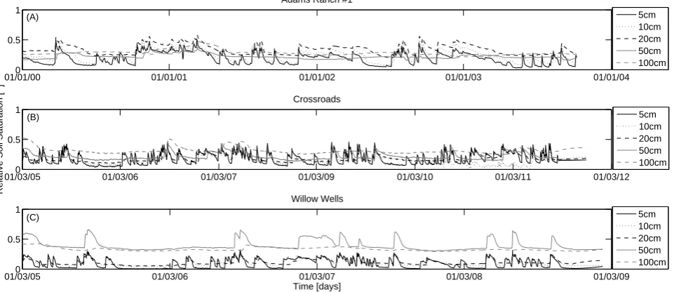
The Soil Climate Analysis Network (SCAN) is composed of more than 190 stations located in 40 states of the US cover-ing different climatic and physical conditions (e.g. Schaefer et al., 2007). It represents an excellent database for the de-scription of the soil moisture and profile under several addi-tional climatic conditions. Measurements are collected with measuring the dielectric devices at approximately 5, 10, 20, 50, and 100 cm depth. For the scope of the paper, we selected three of stations in the state of New Mexico, which is char-acterized by a semiarid climate. The choice was influenced by the opportunity to use the pedological description of the soil column available for these three sites. Such information turned out to be extremely useful for the application of the presented methodology.

The stations selected are Adams Ranch #1, Crossroads, and Willow Wells in New Mexico (US), where continuous soil moisture measurements are available for a period of about 4–5 years. The climatic conditions are quite different from those of the sites in Africa, where we observed a strong seasonal fluctuation in rainfall that is reflected in the dynam-ics of soil moisture. In the present case, this seasonality is limited and in general the soil moisture conditions are drier.

The pedological report available on the web site of SCAN allowed for definition of the soil texture characteristics of the first (the first 10 cm) and the second layer of soil (assumed equal to the remaining 90 cm). We generally found that the upper layer has a higher sand content compared to the lower soil layer. In fact, the second layer of soil was composed of sandy loam in all cases, while the first layer was made of

0 0.2 0.4 0.6 0.8 1

0 0.05 0.1 0.15 0.2 0.25 0.3 0.35

R=0.771

s 1(tj−1) [−]

s 1 (t j−1

)−s

1

(t j

)

(A)

0 0.2 0.4 0.6 0.8 1

0 0.01 0.02 0.03 0.04 0.05 0.06

R=0.834

s 2(tj−1) [−]

s 2 (t j−1

)−s

2

(t j

)

(B)

Fig. 4. Changes in relative soil saturation as a function of the relative

01/01/000 01/01/01 01/01/02 01/01/03 01/01/04 0.5

1

Adams Ranch #1

(A) 5cm

10cm 20cm 50cm 100cm

01/03/050 01/03/06 01/03/07 01/03/09 01/03/10 01/03/11 01/03/12 0.5

1

Relative Soil Saturation [−]

Crossroads

(B) 5cm

10cm 20cm 50cm 100cm

01/03/050 01/03/06 01/03/07 01/03/08 01/03/09 0.5

1

Time [days] Willow Wells

(C) 5cm

10cm 20cm 50cm 100cm

Fig. 5. Time series of the point measurements of the soil relative saturation at the three stations of the SCAN network considered in the

present study: Adams Ranch #1 (A), Crossroads (B), and Willow Wells (C) in New Mexico, US. Probes provide soil moisture measurements at depths ranging from 5 cm down to 100 cm.

sand at Willow Wells and loamy sand at Adams Ranch #1 and Crossroads.

A preliminary description of the soil moisture measure-ments is given in Fig. 5, where the relative saturation of soil at different depths is plotted for these three stations. This plot provides a complete overview on the variability of the soil moisture along the soil column.

4 Model application

4.1 Application on the AMMA database

The SMAR approach was applied to soil measurements available in West Africa, and in particular for the Wankama and Tondikiboro stations in Niger. These soil moisture measurements along with the other point measurements (Nalohou-Mid, Nalohou-Top, and Agoufou) form an excel-lent database that well describes the soil moisture along the root-zone profile. According to this, we have used the sur-face soil moisture measurements at 5 cm depth to predict the soil moisture in the lower layer of the soil, where the relative saturation is measured at various depths.

SMAR contains in total seven parameters (sw2, sc1, Zr1,

Zr2,n1,n2,V2) that can be related to physical characteristics

of the soil profile. All of these parameters can be assigned to four further parameters (a,b,sc1,sw2), as explained in the

previous section. In a preliminary application without cali-bration, we assigned to each of those a value consistent with the physical characteristics of the site under investigation:

– Parameters sw2,sc1,n1, and n2 can be assigned

ac-cording to the soil texture of the site. In particular,

both sites are characterized by sandy soils, and for this reason a first approximation for these parameters can be obtained from values taken from the literature (see characteristics of sand soil in Table 1). In both cases, we assigned the following values:sw2=0.06,

sc1=0.14, n1=0.437, and n2=0.437. Eventually,

the value ofsw2may also be extrapolated by the graph

of Fig. 4a, but in the present case only parameters taken from the literature were adopted.

– Parametera=V2/ (n2Zr2(1−sw))is computed based

on the characteristics of the soil and of the climate. In particular, soil parameters were defined based on the soil texture of the site under investigation, the depth of the second layer of soil, Zr2, was defined

accord-ing to the depth of the deepest probe installed, and, finally, the value of the soil water loss coefficient was defined taking into account both the high permeability of the soil and also the high evapotranspiration losses observed at these specific sites. Consequently, we as-signed the following values for n=0.437 – Zr2=

120 cm at Wankama and 125 cm at Tondikiboro – and V was set equal to 20 mm day−1.

01/01/060 01/01/07 01/01/08 01/01/09 01/01/10 0.2

0.4 0.6 0.8

1 R=0.881, RMSE=0.168, a=0.041, b=0.083, sw2=0.06, sc1=0.14

Relative Soil Saturation [−]

Niger at Wankama

01/01/060 01/01/07 01/01/08 01/01/09 01/01/10

0.2 0.4 0.6 0.8 1

Time [days]

Relative Soil Saturation [−]

Niger at Tondikiboro R=0.856, RMSE=0.203, a=0.037, b=0.08, s_w2=0.06, s_c1=0.14 s

1 s₂

s 2 *

SMAR

s 1 s₂

s 2 *

SMAR (B)

(A)

Fig. 6. Comparison between the relative saturation at 5 cm (s1) and the averaged value over 100, 130, and 135 cm depth, and the filtered

value (s_2SMAR∗ – black line) obtained with SMAR for two sites located at Wankama (A) and Tondikiboro (B), respectively. Results have been obtained assigning parameters based on the physical characteristics of the study cases.

The results of this preliminary application are given in Fig. 6, where one can see the good performance of the method in capturing the trend in the signal of soil mois-ture in the lower soil layer over a temporal window of 4 years. The graph provides a description of the application of SMAR to the two time series measured in Niger with the parameters assigned as described above. The model repro-duces the seasonality of the soil moisture signal very well, with some discrepancies during the transition phases. Cor-relations ofR=0.88 andR=0.85 and a root-mean-square errors (RMSE) of 0.168 and 0.203 are found for Wankama and Tondikiboro stations, respectively.

The same model was also used over several time series available on the AMMA network using the three super sites (Benin, Niger, and Mali) using the averaged values of rela-tive saturation estimated from several point measurements, using all points that provide a complete description of the root profile, and the averaged values estimated over the three super sites (Benin, Niger, and Mali). In fact,t The AMMA network was built with the specific aim to monitor the av-eraged soil moisture over three super sites of 25×25 km2. These data are particularly useful for shedding light on the impact of different scales on the use of SMAR.

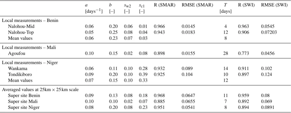
In this case, the model was calibrated for all parameters using the RMSE between the averaged relative saturation of the lower layer of soil and the filtered time series ofs1as an

objective function. This calibration procedure was performed for both the SWI method (optimizing the parameterT) and SMAR (optimizing the parametersa,b,sw2, andsc1),

obtain-ing the results summarized in Table 2. In general, the SMAR procedure produced better results in terms of correlation and RMSE, but this is not surprising considering the number of

parameters in the second equation. Nevertheless, it is encour-aging from our perspective that the calibration parameters are very close to those estimated based on the physical informa-tion available (soil texture, potential evapotranspirainforma-tion, and soil permeability) for the site confirming the physical consis-tency of the methodology.

More specifically, the result of the application of the two procedures for the super sites is given in Fig. 7, where one can see the behaviour of the two expressions when applied to this data set. Apart from the general evaluation of the per-formances that are influenced by the different level of com-plexity of the two schemes, it is interesting to note that the calibrated parameters of SMAR applied to the three super sites are closely related to the values obtained for the point measurements. In particular, it can be observed in Table 1 that the parametersa andsw2 seem to be less sensitive to

the change in scale, while the parametersbandsc1display a

higher variability at the two analysed scales. In general, the calibrated values of the parameters reflect the physical char-acteristics of the sites in terms of soil water losses and other characteristics.

4.2 Application on the SCAN database

01/01/060 01/01/07 01/01/08 01/01/09 31/12/09 0.5

1

SMAR: R=0.968, RMSE=0.0648, a=0.085, b=0.125, s

w2=0.08, sc1=0.175 SWI: R=0.959, RMSE=0.0809, T=11

Super Site Benin

01/01/050 01/01/06 01/01/07 01/01/08 31/12/08 0.5

1

SMAR: R=0.886, RMSE=0.0655, a=0.1, b=0.095, s

w2=0.02, sc1=0.0625 SWI: R=0.892, RMSE=0.0697, T=7

relative soil saturation [−]

Super Site Mali s1

s₂ s₂*

s₂*_SMAR

01/01/060 01/01/07 01/01/08 01/01/09 31/12/09 0.5

1

SMAR: R=0.953, RMSE=0.0530, a=0.0825, b=0.2, s

w2=0.08, sc1=0.225 SWI: R=0.894, RMSE=0.0892, T=8

Time [days] Super Site Niger

(C) (A)

(B)

Fig. 7. Comparison between the relative saturation measured at 5 cm (s1) and the averaged value in the second soil layer of depth (s2), the

filtered value (s_2SMAR∗ ) obtained with SMAR and the filtered value obtained with the exponential filter (s₂∗) for three super sites located respectively in Benin (A), Mali (B), and Niger (C). Results describe the application of SMAR and the exponential filter (SWI) method where all parameters have been calibrated optimizing the RMSE.

Table 2. Summary of the results of the calibration with the SMAR and SWI methods on the time series of the AMMA database analysed

herein.

a b sw2 sc1 R (SMAR) RMSE (SMAR) T R (SWI) RMSE (SWI)

[days−1] [–] [–] [–] [days]

Local measurements – Benin

Nalohou-Mid 0.06 0.20 0.06 0.01 0.966 0.0145 4 0.963 0.0545 Nalohou-Top 0.05 0.25 0.08 0.04 0.943 0.0183 12 0.906 0.07203

Mean values 0.06 0.23 0.07 0.03 8

Local measurements – Mali

Agoufou 0.10 0.15 0.02 0.08 0.898 0.0155 28 0.773 0.0456

Local measurements – Niger

Wankama 0.06 0.11 0.10 0.28 0.932 0.089 14 0.911 0.102 Tondikiboro 0.09 0.20 0.10 0.39 0.925 0.104 10 0.897 0.124

Mean values 0.07 0.15 0.10 0.33 12

Averaged values at 25km×25 km scale

Super site Benin 0.09 0.13 0.08 0.18 0.968 0.0647 11 0.959 0.08 Super site Mali 0.10 0.10 0.02 0.07 0.885 0.0655 7 0.892 0.069 Super site Niger 0.08 0.20 0.08 0.23 0.951 0.0541 8 0.894 0.0891

adopted in the previous section, we assigned the following parameters to three considered case studies:

– Soil parameters were assigned based on the soil

char-acteristics of the sites. We assigned the following soil parameters:

n1=0.437, n2=0.453, sc1=0.24, sw2=0.19,

for Adams Ranch #1;

n1=0.437; n2=0.453; sc1=0.24, sw2=0.19

for Crossroads;

n1=0.437;n2=0.453;sc1=0.14, sw2=0.19

for Willow Wells.

– Considering that the potential evapotranspiration and

soil permeability of these sites may produce values of soil water losses similar to those of the AMMA sites, we assigned the same value ofV2=20 mm day−1.

Pa-rametera was computed using Eq. (2) and adopting the soil parameters derived from the soil texture.

– The parameterb was estimated using Eq. (3) and as-suming the first layer of soil of Zr1=10 cm and the

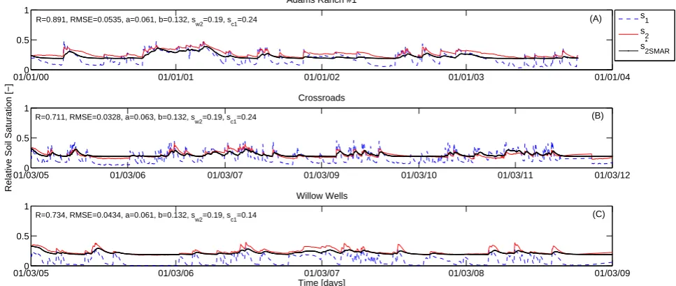
01/01/000 01/01/01 01/01/02 01/01/03 01/01/04 0.5

1

R=0.891, RMSE=0.0535, a=0.061, b=0.132, s

w2=0.19, sc1=0.24

Adams Ranch #1

s₁

s₂ s

2 *

SMAR

01/03/050 01/03/06 01/03/07 01/03/09 01/03/10 01/03/11 01/03/12 0.5

1

R=0.711, RMSE=0.0328, a=0.063, b=0.132, s

w2=0.19, sc1=0.24

Relative Soil Saturation [−]

Crossroads

01/03/050 01/03/06 01/03/07 01/03/08 01/03/09 0.5

1

R=0.734, RMSE=0.0434, a=0.061, b=0.132, s

w2=0.19, sc1=0.14

Time [days] Willow Wells

(A)

(B)

(C)

Fig. 8. Comparison between the relative saturation of the surface soil layer (s1) and the averaged value over 90cm depth (s2), and the filtered

value (s_2SMAR∗ – black line) obtained with SMAR for three sites located at Adams Ranch #1 (A), Crossroads (B), and Willow Wells (C), respectively. Results have been obtained assigning parameters based on the physical characteristics of the study area.

The results of this preliminary application are given in Fig. 8, where one can see the good performance of the method in capturing the trend of the signal of soil mois-ture in the lower soil layer. The graph provides a description of the application of SMAR to the time series measured in New Mexico with the parameters assigned. The application of SMAR without calibration provided encouraging results that are corroborated by the observed correlation coefficients and the RMSE between the observation and the reconstructed values of the relative saturation of the second layer of soil. In particular, we observed a correlation ofR=0.89, 0.71, and 0.73 and a RMSE of 0.053, 0.0328, and 0.0434 for Adams Ranch #1, Crossroads, and Willow Wells stations, respec-tively.

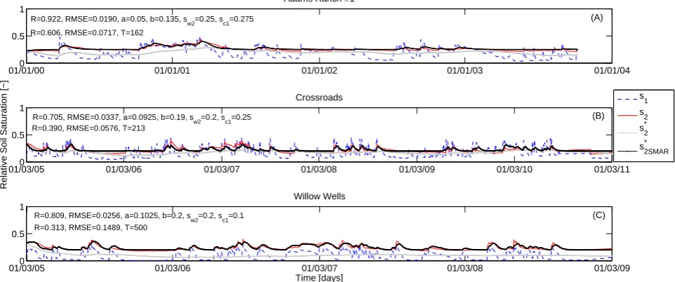
SMAR was also compared with SWI in order to provide a complementary comparison of the performances of the two methods on a different context. Such comparison was carried out with a calibration of both models aimed at the minimiza-tion of the RMSE. The result of the applicaminimiza-tion of the two procedures is shown in Fig. 9 for the three SCAN sites de-scribed. Here the performances of the SMAR algorithm pro-vide an excellent result compared with SWI. Here one may appreciate the performances of the two procedures after cal-ibration.

In addition to the three mentioned stations, we also con-sidered four additional stations in New Mexico where the soil pedon report was not available. For this reason, these data were only used for a comparison with SWI. The re-sults of this application can be found in Table 3 for the soil moisture station of the SCAN network in New Mexico. It can be observed that, apart from the general evaluation of

the performances that are influenced by the different level of complexity of the two schemes, it is interesting to note that SMAR produces better results both in terms ofRvalues and RMSE. Nevertheless, SMAR fails in the interpretation of the soil moisture at the station of Los Lunas, where SWI also performed very poorly. This may be due to errors in the data or in a limitation of the two procedures. In general, the calibrated values of the parameters reflect the physical char-acteristics of the sites in terms of soil water losses and other characteristics.

The analysis presented provides a preliminary comparison between the two methods, highlighting the good performance of SMAR in dry environments. Nevertheless, a more accu-rate/comprehensive intercomparison between the two mod-els could be performed using the AIC and BIC methods (e.g. Ye et al., 2008) to assess model fit, but would be penalized by the number of estimated parameters.

5 Conclusions

In this paper, we introduced a new methodology, named SMAR, for the description of soil moisture in the root zone based on the time series of surface soil moisture data. SMAR has a physically consistent structure, with parameters that may be estimated from the physical characteristics of the site under investigation. Results obtained using as much of the available physical information as possible provided good re-sults.

01/01/000 01/01/01 01/01/02 01/01/03 01/01/04 0.5

1

R=0.922, RMSE=0.0190, a=0.05, b=0.135, s

w2=0.25, sc1=0.275 R=0.606, RMSE=0.0717, T=162

Adams Ranch #1

01/03/050 01/03/06 01/03/07 01/03/08 01/03/09 01/03/10 01/03/11 0.5

1

R=0.705, RMSE=0.0337, a=0.0925, b=0.19, s

w2=0.2, sc1=0.25 R=0.390, RMSE=0.0576, T=213

Relative Soil Saturation [−]

Crossroads s

1

s₂

s₂*

s₂*_SMAR

01/03/050 01/03/06 01/03/07 01/03/08 01/03/09 0.5

1

R=0.809, RMSE=0.0256, a=0.1025, b=0.2, s

w2=0.2, sc1=0.1 R=0.313, RMSE=0.1489, T=500

Time [days] Willow Wells

(A)

(B)

(C)

Fig. 9. Comparison between the relative saturation of the surface soil layer (s1) and the averaged value over the first 90 cm of depth (s2),

the filtered value (s_2SMAR∗ ) obtained with SMAR and the filtered value obtained with the exponential filter (s₂∗) for three sites located at Adams Ranch #1 (A), Crossroads (B), and Willow Wells (C), respectively. Results describe the application of SMAR and the exponential filter (SWI) method, where all parameters have been calibrated optimizing the RMSE.

Table 3. Summary of the results of the calibration with the SMAR and SWI methods on the time series of the SCAN database.

Station a b sw2 sc1 R (SMAR) RMSE (SMAR) T R (SWI) RMSE (SWI)

[days−1] [–] [–] [–] [days]

Adams Ranch #1 0.05 0.14 0.25 0.28 0.92 0.02 162 0.61 0.07 Alcalde 0.06 0.05 0.23 0.24 0.91 0.02 43 0.81 0.07 Crossroads 0.09 0.19 0.20 0.25 0.76 0.03 73 0.62 0.05 Jordana Exp. Range 0.05 0.05 0.05 0.01 0.88 0.02 59 0.88 0.04 Los Lunas 0.05 0.20 0.33 0.29 0.36 0.08 500 −0.59 0.19 Sevilleta 0.05 0.17 0.23 0.18 0.81 0.03 500 0.68 0.14 Willow Wells 0.08 0.20 0.20 0.13 0.90 0.02 189 0.45 0.14

measurements, SMAR has been applied using available in-formation in order to infer parameter values. The prelimi-nary application carried out without the need of calibration provided a satisfying result both in terms ofR values and RMSE. In order to explore the potential of this new formu-lation, its performances have been compared with the results obtained through the simple exponential filter proposed by Wagner et al. (1999). Both methods have been used after cal-ibration on several time series of the AMMA and the SCAN. The comparison highlighted that this procedure may provide some improvements in semiarid environments. Moreover, the set of parameters obtained from calibration is consistent with the physical characteristics of the studied area.

The proposed method may be improved by including a soil loss function that accounts for the non-linearity of this pro-cess. This step is straightforward, but will incorporate a sig-nificant number of additional parameters in the proposed

re-lationship, while in the present form the equation provides an interesting, descriptive functional relationship between two variables of extreme interest.

Acknowledgements. The authors wish to acknowledge Wolfgang

Wagner and the second, anonymous reviewer for their stimulating comments. Moreover, we are particularly grateful to Thierry Pellarin for his valuable help in providing us all the necessary data for the study. Finally, we take this opportunity to remember the co-author Florisa Melone, who sadly passed away on 28 October 2012. Our sole consolation is that we had the honour and privilege of working with her, but even more the joy of her friendship.

References

Albergel, C., Rüdiger, C., Pellarin, T., Calvet, J.-C., Fritz, N., Frois-sard, F., Suquia, D., Petitpa, A., Piguet, B., and Martin, E.: From near-surface to root-zone soil moisture using an exponential fil-ter: an assessment of the method based on in-situ observations and model simulations, Hydrol. Earth Syst. Sci., 12, 1323–1337, doi:10.5194/hess-12-1323-2008, 2008.

Albergel, C., Dorigo, W., Balsamo, G., Muñoz-Sabater, J., de Ros-nay, P., Isaksen, L., Brocca, L., de Jeu, R., and Wagner, W.: Mon-itoring multi-decadal satellite earth observation of soil moisture products through land surface reanalyses, Remote Sens. Envi-ron., 138, 77–89, doi:10.1016/j.rse.2013.07.009, 2013.

AMMA: AMMA-CATCH, 2014: Hydrological and meteorolog-ical observatory on West Africa, available at: http://www. amma-catch.org, last access: December 2013, 2014.

AMMA Database: AMMA Data User Interface, available at: http: //database.amma-international.org/, last access: December 2013, 2014.

Brocca, L., Melone, F., Moramarco, T., Wagner, W., Naeimi, V., Bartalis, Z., and Hasenauer, S.: Improving runoff prediction through the assimilation of the ASCAT soil moisture product, Hydrol. Earth Syst. Sci., 14, 1881–1893, doi:10.5194/hess-14-1881-2010, 2010.

Brocca, L., Moramarco, T., Melone, F., Wagner, W., Hasenauer, S., and Hahn, S.: Assimilation of surface and root-zone ASCAT soil moisture products into rainfall-runoff modelling, IEEE T. Geosci. Remote, 50, 2542–2555, 2012.

Brooks, R. H. and Corey A. T.: Hydraulic properties of porous me-dia, Hydrol. Pap. 3, Colorado State Univ., Fort Collins, USA, 1964.

Ceballos, A., Scipal, K., Wagner, W., and Mart?nez-Fernandez, J.: Validation of ERS Scatterometer-Derived Soil Moisture Data in the Central Part of the Duero Basin, Spain, Hydrol. Process., 19, 1549–1566, 2005.

Crow, W. T., Kustas, W. P., and Prueger, J. H.: Monitoring root-zone soil moisture through the assimilation of a thermal remote sensing-based soil moisture proxy into a water balance model, Remote Sens. Environ., 112, 1268–1281, 2008.

De Lange, R., Beck, R., Van De Giesen, N., Friesen, J., De Wit, A., and Wagner, W.: Scatterometer-derived soil moisture cal-ibrated for soil texture with a onedimensional water-flow model, IEEE Trans. Geosci. Remote Sens., 46, 4041–4049, doi:10.1109/TGRS.2008.2000796, 2008.

de Rosnay, P., Gruhier, C., Timouk, F., Baup, F., Mougin, E., Hier-naux, P., Kergoat, L., and LeDantec, V.: Multi-scale soil moisture measurements at the Gourma meso-scale site in Mali, J. Hydrol., 375, 241–252, 2009.

Dorigo, W. A., Wagner, W., Hohensinn, R., Hahn, S., Paulik, C., Xaver, A., Gruber, A., Drusch, M., Mecklenburg, S., van Oeve-len, P., Robock, A., and Jackson, T.: The International Soil Mois-ture Network: a data hosting facility for global in situ soil mois-ture measurements, Hydrol. Earth Syst. Sci., 15, 1675–1698, doi:10.5194/hess-15-1675-2011, 2011.

Escorihuela, M., Chanzy, A., Wigneron, J., and Kerr, Y.: Effective soil moisture sampling depth of L-band radiometry: a case study, Remote Sens. Environ., 114, 995–1001, 2010.

Gao, H., Wood, E. F., Jackson, T. J., Drusch, M., and Bindlish, R.: Using TRMM/TMI to Retrieve Surface Soil Moisture over the

Southern United States from 1998 to 2002, J. Hydrometeorol., 7, 23–38, 2006.

Green, W. H. and Ampt, G.: Studies of soil physics, part I – the flow of air and water through soils, J. Agr. Sci., 4, 1–24, 1911. ISMN (International Soil Moisture Network): The ISMN Data

Por-tal, available at: http://ismn.geo.tuwien.ac.at, last access: Decem-ber 2013, 2014.

Laio, F.: A vertically extended stochastic model of soil mois-ture in the root zone, Water Resour. Res., 42, W02406, doi:10.1029/2005WR004502, 2006.

Li, F., Crow, W. T., and Kustas, W. P.: Towards the estimation of root-zone soil moisture via the simultaneous assimilation of ther-mal and microwave soil moisture retrievals, Adv. Water Resour., 33, 201–214, 2010.

Liang, X., Lettenmaier, D. P., Wood, E. F., and Burges, S. J.: A sim-ple hydrologically based model of land surface water and energy fluxes for GCMs, J. Geophys. Res., 99, 14415–14428, 1994. Liang, X., Lettenmaier, D. P., and Wood, E. F.: One-dimensional

statistical dynamic representation of subgrid spatial variability of precipitation in the two-layer variable infiltration capacity model, J. Geophys. Res., 101, 21403–21422, 1996.

Manfreda, S. and Fiorentino, M.: A stochastic approach for the de-scription of the water balance dynamics in a river basin, Hy-drol. Earth Syst. Sci., 12, 1189–1200, doi:10.5194/hess-12-1189-2008, 2008.

Manfreda, S., McCabe, M., Wood, E. F., Fiorentino, M., and Rodriguez-Iturbe, I.: Spatial Patterns of Soil Moisture from Dis-tributed Modeling, Adv. Water Resour., 30, 2145–2150, 2007. Manfreda, S., Lacava, T., Onorati, B., Pergola, N., Di Leo, M.,

Mar-giotta, M. R., and Tramutoli, V.: On the use of AMSU-based products for the description of soil water content at basin scale, Hydrol. Earth Syst. Sci., 15, 2839–2852, doi:10.5194/hess-15-2839-2011, 2011.

Matgen, P., Heitz, S., Hasenauer, S., Hissler, C., Brocca, L., Hoff-mann, L., Wagner, W., and Savenije, H. H. G.: On the potential of METOP ASCAT-derived soil wetness indices as a new aper-ture for hydrological monitoring and prediction: a field evalua-tion over Luxembourg, Hydrol. Process., 26, 2346–2359, 2012a. Matgen, P., Fenicia, F., Heitz, S., Plaza, D., de Keyser, R., Pauwels, V. R. N., Wagner, W., and Savenije, H.: Can ASCAT-derived soil wetness indices reduce predictive uncertainty in well-gauged ar-eas? A comparison with in situ observed soil moisture in an as-similation application, Advances in Water Resources, 44, 49–65, doi:10.1016/j.advwatres.2012.03.022, 2012b.

Moran, M. S., Peters-Lidard, C. D., Watts, J. M., and McElroy, S.: Estimating soil moisture at the watershed scale with satellite-based radar and land surface models, Can. J. Remote Sens., 30, 805–826, 2004.

Nied, M., Hundecha, Y., and Merz, B.: Flood-initiating catchment conditions: a spatio-temporal analysis of large-scale soil mois-ture patterns in the Elbe River basin, Hydrol. Earth Syst. Sci., 17, 1401–1414, doi:10.5194/hess-17-1401-2013, 2013. Ochsner, T., Cosh, M., Cuenca, R., Dorigo, W., Draper, C.,

Hag-imoto, Y., Kerr, Y., Larson, K. M., Njoku, E. G., Small, E. E., and Zreda, M.: The state of the art in large-scale soil moisture monitoring, Soil Sci. Soc. Am. J., 77, 1888– 1919,doi:10.2136/sssaj2013.03.0093, 2013.

Water Resour. Res., 39, 1314, doi:10.1029/2003WR002142, 2003.

Pellarin, T., Laurent, J. P., Cappelaere, B., Decharme B., Descroix, L., and Ramier, D.: Hydrological modelling and associated mi-crowave emission of a semi-arid region in South-western Niger, J. Hydrol., 375, 262–272, 2009a.

Pellarin, T., Tran, T., Cohard, J.-M., Galle, S., Laurent, J.-P., de Ros-nay, P., and Vischel, T.: Soil moisture mapping over West Africa with a 30-min temporal resolution using AMSR-E observations and a satellite-based rainfall product, Hydrol. Earth Syst. Sci., 13, 1887–1896, doi:10.5194/hess-13-1887-2009, 2009b. Porporato, A., Daly, E., and Rodriguez-Iturbe, I.: Soil water balance

and ecosystem response to climate change, Am. Nat., 164, 625– 632, 2004.

Puma, M. J., Celia, M. A., Rodriguez-Iturbe, I., and Guswa, A. J.: Functional relationship to describe temporal statistics of soil moisture averaged over different depths, Adv. Water Resour., 28, 553–566, 2005.

Ragab, R.: Towards a continuous operational system to estimate the root zone soil moisture from intermittent remotely sensed surface moisture, J. Hydrol., 173, 1–25, 1995.

Rawls, W. J. and Brakensiek D. L.: Estimation of soil water re-tention and hydraulic properties, in: Unsaturated Flow in Hy-drologic Modeling, Kluwer Acad., Dordrecht, Netherlands, 275– 300, 1989.

Rawls, W. J., Ahuja, L. R., Brakensiak, D. L., and Shirmohammadi, A.: Infiltration and soil water movement, in: Handbook of Hy-drology, edited by: Maidment, D. R., 5.1–5.51, 1993.

Redelsperger, J.-L., Thorncroft, C. D., Diedhiou, A., Lebel, T., Parker, D., and Polcher, J.: African Monsoon Multidisciplinary Analysis: An International Research Project and Field Cam-paign, B. Am. Meteorol. Soc., 87, 1739–1746, 2006.

Reichle, R., McLaughlin, D., and Entekhabi, D.: Hydrologic data assimilation with the ensemble kalman filter, Mon. Weather Rev., 130, 103–114, 2002.

Reichle, R., Koster, R., Dong, J., and Berg, A.: Global soil mois-ture from satellite observations, land surface models, and ground data: implications for data assimilation, J. Hydrometeorol., 5, 430–442, 2004.

Rodriguez-Iturbe, I., Isham, V., Cox, D. R., Manfreda, S., and Por-porato, A.: Space-time modeling of soil moisture: stochastic rain-fall forcing with heterogeneous vegetation, Water Resour. Res., 42, W06D05, doi:10.1029/2005WR004497, 2006.

Sabater, J. M., Jarlan, L., Calvet, J. C., Bouyssel, F., and De Rosnay, P.: From Near-Surface to Root-Zone Soil Moisture Using Dif-ferent Assimilation Techniques, J. Hydrometeorol., 8, 194–206, 2007.

Schaefer, G. L., Cosh, M. H., and Jackson, T. J.: The USDA Natural Resources Conservation Service Soil Climate Analysis Network (SCAN), J. Atmos. Ocean. Tech., 24, 2073–2077, 2007. Scipal, K., Drusch, M., and Wagner, W.: Assimilation of a ERS

scat-terometer derived soil moisture index in the ECMWF numerical weather prediction system, Adv. Water Resour., 31, 1101–1112, 2008.

Seneviratne, S. I., Corti, T., Davin, E. L., Hirschi, M., Jaeger, E. B., Lehner, I., Orlowsky, B., and Teuling, A. J.: Investigating soil moisture-climate interactions in a changing climate: A review, Earth-Sci. Rev., 99, 125–161, 2010.

Wagner, W., Lemoine, G., and Rott, H.: A method for estimat-ing soil moisture from ERS scatterometer and soil data, Remote Sens. Environ., 70, 191–207, 1999.

Walker, J. P. and Houser, P. R.: Requirements of a global near-surface soil moisture satellite mission: accuracy, repeat time, and spatial resolution, Adv. Water Resour., 27, 785–801, 2004. Wood, E. F., Lettenmaier, D. P., Liang, X., Nijssen, B., and Wetzel,

S. W.: Hydrological modeling of continental-scale basins, Annu. Rev. Earth Pl. Sc., 25, 279–300, 1997.