Understanding how ESOL Pre Services Teachers' Prior Experiences and Background Shape their Processes of becoming L2 (Reading) Teachers

ScholarWorks @ Georgia State University

ScholarWorks @ Georgia State University

Economics Dissertations

Summer 8-11-2011

Essays on Fiscal Policy and Economic Growth

Essays on Fiscal Policy and Economic Growth

Tamoya A. L. Christie

Georgia State University

Follow this and additional works at: https://scholarworks.gsu.edu/econ_diss

Part of the Economics Commons

Recommended Citation Recommended Citation

Christie, Tamoya A. L., "Essays on Fiscal Policy and Economic Growth." Dissertation, Georgia State University, 2011.

https://scholarworks.gsu.edu/econ_diss/75

In presenting this dissertation as a partial fulfillment of the requirements for an advanced degree from Georgia State University, I agree that the Library of the University shall make it available for inspection and circulation in accordance with its regulations governing materials of this type. I agree that permission to quote from, to copy from, or to publish this dissertation may be granted by the author or, in his or her absence, the professor under whose direction it was written or, in his or her absence, by the Dean of the Andrew Young School of Policy Studies. Such quoting, copying, or publishing must be solely for scholarly purposes and must not involve potential financial gain. It is understood that any copying from or publication of this dissertation which involves potential gain will not be allowed without written permission of the author.

All dissertations deposited in the Georgia State University Library must be used only in accordance with the stipulations prescribed by the author in the preceding statement.

The author of this dissertation is:

Tamoya A.L. Christie 280 Winona Dr. Garvey Meade Bridgeport P.O.

Portmore, St. Catherine Jamaica, W.I.

The director of this dissertation is:

Felix K. Rioja Economics

Andrew Young School of Policy Studies Georgia State University

P. O. Box 3992

Atlanta, GA 30302-3992

Users of this dissertation not regularly enrolled as students at Georgia State University are required to attest acceptance of the preceding stipulations by signing below. Libraries borrowing this dissertation for the use of their patrons are required to see that each user records here the information requested.

Type of use

ESSAYS ON FISCAL POLICY AND ECONOMIC GROWTH

BY

TAMOYA A.L. CHRISTIE

A Dissertation Submitted in Partial Fulfillment of the Requirements for the Degree

of

Doctor of Philosophy in the

Andrew Young School of Policy Studies of

Georgia State University

Copyright by Tamoya A.L. Christie

This dissertation was prepared under the direction of the candidate’s Dissertation Committee. It has been approved and accepted by all members of that committee, and it has been accepted in partial fulfillment of the requirements for the degree of Doctor of Philosophy in Economics in the Andrew Young School of Policy Studies of Georgia State University.

Dissertation Chair: Felix K. Rioja

Committee: Shiferaw Gurmu

Jenny E. Ligthart

Jorge Martinez-Vazquez Neven T. Valev

Electronic Version Approved:

Mary Beth Walker, Dean

Andrew Young School of Policy Studies Georgia State University

vi

I am grateful to the members of my dissertation committee for insightful

comments and guidance. I would also like to thank Dr. David Sjoquist who has

consistently given encouragement in my research endeavors. Finally, I would like to

acknowledge my husband and my family who never wavered in their support and

vii

ACKNOWLEDGMENTS ... vi

LIST OF TABLES ... ix

LIST OF FIGURES ... x

ABSTRACT ... xi

INTRODUCTION ... 1

ESSAY 1 ... 6

THE EFFECT OF GOVERNMENT SPENDING ON ECONOMIC GROWTH: ... 6

Introduction ... 6

Data and Empirical Methodology ... 11

Data ... 11

Model Specification and Estimation ... 13

Results ... 16

Threshold Existence ... 16

Threshold Effects ... 18

Sensitivity Analysis ... 24

Conclusion ... 26

ESSAY 2 ... 29

FINANCING PRODUCTIVE GOVERNMENT EXPENDITURES: ... 29

Introduction ... 29

Literature Review... 34

The Theoretical Model ... 39

Households ... 40

Producers... 43

The Government ... 45

Equilibrium Conditions and the Balanced Growth Path ... 46

Model Calibration and Solution ... 49

Policy Experiments ... 51

The Region Average ... 53

Fiscal Strategy under Different Initial Fiscal Conditions ... 58

viii

APPENDIX A ... 79

APPENDIX B ... 87

REFERENCES ... 88

ix

Table Page

1 Descriptive Statistics, 1971-2005………... 67

2 Threshold Identification and Inference ……….. 68

3 Baseline Regression Results ……….. 68

4 GMM Estimation to Address Endogeneity ……… 69

5 Productive Government Spending ………. 70

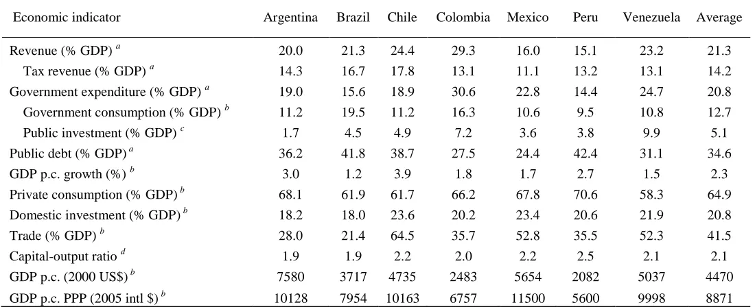
6 Selected Economic Indicators 1990-2008 ………. 71

7 Benchmark Parameters for Region Average ………. 72

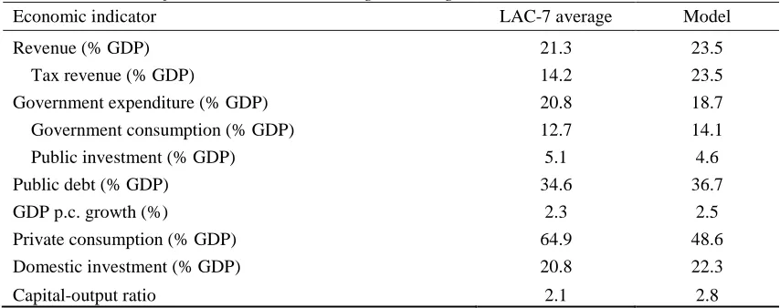
8 Benchmark Solution for Model Calibrated to Region Average ……… 72

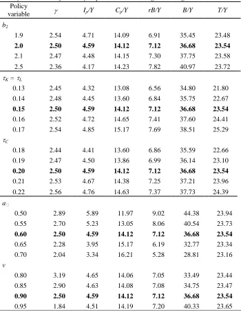
9 Steady-State Results for Policy Experiments on the Region Average …….. 73

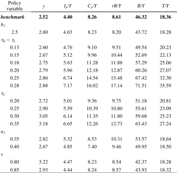
10 Steady-State Results for ―High Debt, High Tax‖ Scenario ………... 74

11 Steady-State Results for ―Low Debt, Low Tax‖ Scenario ………. 75

x

Figure Page

1 Over time averages of government size relative to GDP per capita

growth by country………... 77

2 Distribution of estimation observations according to government size

and GDP growth ………. 77

3 LR1 statistics and confidence intervals for threshold inference

xi

ESSAYS ON FISCAL POLICY AND ECONOMIC GROWTH

By

TAMOYA A.L. CHRISTIE

August 2011

Committee Chair: Dr. Felix Rioja

Major Department: Economics

This dissertation comprises two essays that elaborate on different aspects of the

relationship between government expenditure and long-term economic growth. The first

essay explores how the size of government, as measured by the level of spending, affects

growth. Theoretical models suggest a nonlinear relationship; however, testing this

hypothesis empirically in cross-country studies is complicated by the endogeneity of

government spending and the accurate identification of turning points. This paper

examines the nonlinear hypothesis by incorporating threshold analysis in a cross-country

growth regression. The methodology utilizes a sample-splitting framework and follows

an objective strategy for identifying and testing changes in the slope. Using a broad panel

of countries over the period 1971-2005, the results show evidence in favor of a nonlinear

effect, but not of the form predicted by theory. When total government spending is low,

there is no statistically significant effect on economic growth. However, after passing a

certain threshold (26 percent for developed countries and 33 percent for developing

countries) government spending exhibits a negative effect on growth. This pattern

xii

variations in the composition and financing of government expenditures affect economic

growth in the long-run. The model is used to analyze how public investment spending

funded by taxes or borrowing affects long-term output growth. We also examine the

effect of varying the composition of public expenditure, shifting between consumption

and investment spending, or re-allocating between different types of public investment.

In addition, we use alternative parameterizations of the model to explore how the effects

on growth change under extreme initial fiscal conditions such as high average tax rates,

debt ratios and public consumption spending. The model is calibrated to reflect economic

conditions in the seven largest Latin American economies during the period 1990 to

2008. We find that, where tax rates are not already high, funding public investment by

raising taxes may increase long-run growth. If existing tax rates are high, then public

investment is only growth-enhancing if funded by restructuring the composition of public

spending. Interestingly, using debt to finance new public investment compromises

INTRODUCTION

The general increase in the average size of government over time has precipitated

fears that progressively larger governments will compromise economic growth. This has

prompted calls to scale back government activities and cut budgets. However, the areas

of government spending which typically end up being cut during fiscal adjustment are

categories associated with productive expenditure—public investment in physical

infrastructure, education and healthcare, for example. Spending in these areas has been

shown to have a positive impact on aggregate production and is considered crucial for

long-term growth and development. Policymakers risk doing more harm than good to

their economies over the long-run if the appropriate level and composition of public

expenditure is not maintained.

Of course, one of the major challenges facing governments is how to finance such

expenditures given binding fiscal constraints. Moreover, it has been shown that diverse

types of government expenditure may have conflicting effects on growth given different

sources of financing. Income taxes tend to be distortionary creating disincentives to

saving and investment, while deficit financing may crowd out private investment

(Agénor, 2004; Kneller, Bleaney, & Gemmell, 1999). It is therefore also important to

know how government spending can be most efficiently allocated and financed to bring

about the best growth results, particularly in the context of adverse fiscal conditions such

as already high tax rates, large fiscal deficits and growing debt stocks.

This dissertation comprises two essays that examine different aspects of the

relationship between government spending and long-term economic growth. The first

essay explores the topical issue of size, as measured by the level of government spending

stipulates there is a nonlinear relationship between government size and economic

growth; such that government spending is enhancing at low levels but

growth-retarding at high levels, with the optimal size occurring somewhere in between. The

second essay complements the first by delving into issues concerning the optimal

composition and financing of public expenditures, and how these vary depending on

heterogeneous fiscal conditions across countries. The premise is that the appropriate

fiscal strategy in one country may not be the same in another where fiscal conditions are

more stringent.

In the first essay, the objective of empirically testing the nonlinear hypothesis in

cross-country studies is complicated by the endogeneity of government spending and the

accurate identification of turning points. We attempt to overcome these problems and in

so doing make several contributions to the existing literature. First, in terms of

methodology, we incorporate threshold analysis in the cross-country growth regression.

This methodology utilizes a sample-splitting framework and follows an objective strategy

for identifying and testing changes in the slope. In addition, we apply generalized method

of moments (GMM) dynamic panel techniques to address potential endogeneity of

government expenditure. Second, with respect to data, we employ an updated data set

with a broad cross-section of countries over a long time span. Pulling data from the

International Monetary Fund’s (IMF) Government Finance Statistics (GFS), the sample

contains 136 countries over the period 1971-2005. Most important, this data source offers

a more comprehensive measure of government size by using total government

expenditure (excluding interest payments) as opposed to government consumption

studies, does not include public capital formation and so cannot fully capture the

productivity-enhancing effects of government services. Moreover, the GFS data contain

sectoral decompositions of government spending, which allows us to isolate ―productive‖

as opposed to ―unproductive‖ elements of government spending from the total. This

enables us to also explore, in broad terms, different effects due to the composition of

public spending.

We find evidence to support a nonlinear effect, but not of the form suggested by

the nonlinear hypothesis. For total government spending above a critical size threshold,

we find a negative effect on growth. However, this effect is negligible for government

size below the threshold, and only displays a positive—though not statistically

significant—coefficient when productive government spending is distinguished from the

total. We also find evidence to suggest that other factors may affect the nature of the

relationship between government size and growth. The level of economic development

and the quality of government are two such factors. When we analyze developed and

developing countries separately, the threshold location is lower for developed countries.

In addition, high quality governance mitigated some of the negative effects so that

nonlinearities were more pronounced in countries with less effective governments.

The findings of this study have significant public policy implications as they offer

some insight to the policy debate about the optimal size of government, and how this

varies according to the level of economic development of a country. Indeed, the concern

about large governments is not misplaced as several countries have exceeded the critical

threshold identified in this study. Further expansion of government will have negative

improvements to the quality of government can dampen these negative effects. On

another note, the negligible growth effects of government spending below the threshold

imply serious offsetting influences, which mitigate the potential benefits from increased

public spending. The extent to which the mitigating factors are due to the composition

and financing of public expenditures is explored in the second essay.

The second essay of the dissertation develops a two-sector endogenous growth

model which is capable of explaining how variations in the composition and financing of

government expenditures affect economic growth rates in the long-run. The model is

used to analyze how public investment spending funded by taxes (income or

consumption) or by borrowing affects long-term output growth. We also examine the

effect of varying the composition of public expenditure, shifting the proportions of

productive versus unproductive spending, or re-allocating between different types of

productive expenditure. In addition, we explore how heterogeneous fiscal conditions

affect the implications for growth. Specifically, we use alternative parameterizations of

the model to simulate extreme initial fiscal conditions such as high average tax rates, debt

stock ratios and government consumption spending. The implications of the model are

tested using quantitative methods. The model is calibrated to reflect economic conditions

in the seven largest Latin American economies during the period 1990 to 2008. The Latin

American countries provide a suitable testing ground given their debt history and diverse

fiscal adjustment experiences.

The study makes several contributions to the existing literature. First, we take into

account that government expenditure is not homogenous and spending in different sectors

categorizing government spending merely as ―productive‖ or ―unproductive‖ and

explicitly recognize the heterogeneity within productive government expenditure itself.

To do this, we develop a two-sector endogenous growth model in which public

investment is divided between physical and human capital, allowing for distinct output

effects from each type of spending. Second, the theoretical model moves away from the

balanced government budget constraint typical of the literature and opens up the revenue

options of the government to include deficit financing. This more realistically captures

the actual situation of the majority of economies today and allows us to explore the extent

to which variations in the sources of financing affect the relationship between

government spending and long-term growth. Third, we pay particular attention to how

these effects change under different initial fiscal conditions (such as high tax rates and

large debt stocks), an aspect not previously explored in the growth literature.

We find that the effect of productive government spending on growth is not

necessarily positive, but varies with the overall structure of total public expenditure, the

method of funding and the existing fiscal conditions. This helps to explain the negligible

effect of government spending below the threshold found in the first essay. If existing tax

rates are high, then funding productive spending by further increases in the tax rate,

actually lowers long-run growth. In this case, public investment is only growth-enhancing

if financed by restructuring the composition of public spending. Interestingly, using debt

to finance new public investment compromises growth in the long-run, regardless of the

initial fiscal condition.

The dissertation proceeds with a more detailed discussion of each of the two

ESSAY 1

THE EFFECT OF GOVERNMENT SPENDING ON ECONOMIC GROWTH:

TESTING THE NONLINEAR HYPOTHESIS

Introduction

There has been ongoing concern that large and growing governments have

deleterious effects on the long-run growth of their economies. The usual policy

prescription calls for a scaling back of government activity and budgets, constraining

public spending from growing faster than output. In countries facing fiscal imbalances

and high debt burdens, this has prompted wide-ranging fiscal consolidation programs to

reduce government spending (IMF, 2003). However, parallel to this thrust has been a call

for ―fiscal space‖ in which governments argue for room in their budgets to allow for the

provision of productive public goods that will foster economic growth (Heller, 2005).1

These opposing policies are based on conflicting views on the role of government in the

development process.

The theoretical literature offers support for both positive and negative effects of

government size on economic growth. Government provision of public goods such as

infrastructure, rule of law, and protection of property rights—the core areas of

government – is thought to be conducive to growth (Aschauer, 1989; Ram, 1986).

However, as the size of government increases, distortionary effects of high taxes and

public borrowing, diminishing returns to public capital, rent-seeking activities and

bureaucratic inefficiencies become more prevalent. Public choice theorists argue that

1 _{Productive government expenditure may include, inter alia, spending on highways, roads, education,}

eventually the latter factors dominate and marginal government expenditure exerts a

negative effect on growth (Barth, Keleher, & Russek, 1990; Gwartney, Lawson, &

Holcombe, 1998).

These ideas have been formalized in the endogenous growth literature. Barro

(1990) introduces a non-monotonic relationship through the rising distortionary effect of

increasing tax rates which are required to fund ever larger government expenditure. In the

Barro model, when government is relatively small, growth rises with increases in

productive government services as the positive effects of more public goods dominates,

but beyond some critical point the disincentive effects of higher taxes on savings and

investment reduce the growth rate. If the nonlinear hypothesis is valid and the effect of

government spending on long-run economic growth does vary with its size, this would

not only help to explain the ambiguous findings in the empirical growth literature, but

would also offer clearer guidelines on the appropriate fiscal policy prescription for a

country of a particular government size. Furthermore, implicit in the nonlinear hypothesis

is the existence of some optimal size of government which would maximize economic

growth. Having an indication of this hypothetical optimum, and where a country stands

relative to it, should be of potential interest to policymakers. It must be noted, of course,

that the optimal point is likely to differ for each country depending on various factors

which may attentuate or accentuate the break point. Some factors we are able to control

for, while others we are not.

This chapter tests the validity of Barro’s nonlinear hypothesis on the relationship

between government spending and economic growth. Currently, there is no clear

growth.2 This may be attributable to the fact that the possibility of a nonlinear

relationship has been largely ignored. Those studies which have tried to incorporate a

possible nonlinear effect have been mainly limited to single-country investigations, using

time series data (Chen & Lee, 2005; Grossman, 1988; Mittnik & Neumann, 2003; Vedder

& Gallaway, 1998). Among the relatively few cross-country studies that have explored a

non-monotonic relationship (Afonso & Furceri, 2010; Kelly, 1997; Park, 2006), the

tendency is to include a quadratic term, which usually fails to detect any evidence of

nonlinear effects in the relationship. This may be attributable to the fact that a quadratic

specification assumes one particular form of nonlinearity, but the true effect may be

present in other forms not appropriately modeled by a quadratic term.

Nevertheless, some early evidence in favor of the nonlinear hypothesis using

cross-country data has been provided by Sheehey (1993) and Karras (1996). By dividing

a broad sample of 102 countries according to the initial size of government, Sheehey

finds that increasing the share of government spending to GDP has a positive (negative)

effect on growth when the initial government expenditure share is below (above) 15

percent.3 While these findings are consistent with the nonlinear hypothesis, the choice of

a 15 percent government share threshold is arbitrary, which creates uncertainty about the

correct identification of the growth-maximizing point. Karras takes a different approach

to the nonlinearity question. Although he does not directly test the relationship between

government size and growth, his methodology allows him to determine the productivity

2

Ram (1986) and Rubinson (1977) are among the few who find clear evidence in favor of a positive relationship. Barro (1989) and Kormendi and Meguire (1986) find no significant relationship. On the other hand, studies which find a negative effect include Afonso and Furceri (2010), Folster and Henrekson (2001), Grier and Tullock (1987) and Landau (1983).

3 _{Sheehey (1993) also searches for nonlinearities in government spending on the basis of economic}

of government spending and identify whether or not government services are optimally

provided.4 Moreover, he is able to test the relationship between the marginal productivity

of government services and government size. He finds this relationship to be negative,

implying that the public sector is more productive when small—a feature consistent with

the nonlinear hypothesis.5

More recently, Varoudakis, Tiongson, and Pushak (2007) also investigate the

nonlinear hypothesis for a group of 25 transition economies between 1992 and 2004.

Using spline regressions, they experimented with a number of plausible threshold values

for government size. They eventually settle on a threshold value of 35 percent, which is

approximately equal to the sample median. They find that at expenditure levels of 35

percent of GDP or higher, public spending negatively affects growth. However, at levels

below 35 percent, public sector size had no robust measurable effect.

This chapter re-examines the relationship between government size and long-run

economic growth, explicitly accounting for the likelihood of a nonlinear effect. We

contribute to the literature in a number of ways. First, in terms of methodology, we make

improvements to previous empirical studies by applying threshold analysis (Hansen,

2000) to a panel of 136 countries. This technique has been widely used as the preferred

method to identify threshold effects (Adam & Bevan, 2005; Chen & Lee, 2005; Falvey,

Foster, & Greenaway, 2006; Haque & Kneller, 2009; Khan & Senhadji, 2001),

particularly when the variable of interest is observable, but the position of the threshold is

not known. The methodology uses a sample-splitting framework and follows an objective

4

Karras (1996) takes advantage of the ―Barro rule‖ which states that government services are optimally provided when their marginal product equals unity.

5 _{Furthermore, he calculates the optimal government size to be 23 percent for the average country in his}

strategy for identifying and testing changes in the slope. One important advantage of

threshold analysis is that it avoids the ad hoc, subjective pre-selection of threshold

values—a major critique of previous studies. In addition, we also apply generalized

method of moments (GMM) dynamic panel techniques to address potential endogeneity

of government expenditure, which is measured as a share of GDP. Second, with respect

to data, we employ an updated data set with a broad cross-section of countries over a long

time span. Pulling data from the IMF’s Government Finance Statistics (GFS), our sample

contains 136 countries over the period 1971-2005. Most important, this data source offers

a more comprehensive measure of government size by using total government

expenditure (excluding interest payments) as opposed to government consumption

expenditure as the proxy. The consumption measure, though widely used in empirical

studies, does not include public capital formation and so cannot fully capture the

productivity-enhancing effects of government services. Moreover, the GFS data contain

sectoral decompositions of government spending, which allows us to isolate ―productive‖

as opposed to ―unproductive‖ elements of government spending from the total. This

enables us to also explore, in broad terms, different effects due to the composition of

public spending.

The results of the study suggest evidence in favor of a nonlinear effect, but not as

predicted by Barro’s nonlinear hypothesis (Barro, 1990). When total government

spending is low, we find no statistically significant effect on economic growth. However,

after passing a certain threshold (26 percent for developed countries and 33 percent for

developing countries) government spending exhibits a strong negative effect on growth.

is singled out. The results are qualitatively robust to various specifications and estimation

techniques.

The chapter proceeds as follows. The next section provides a description of the

data and the empirical methodology used in the analysis. The results are discussed in the

third section. Finally, we summarize the findings and conclude with some policy

implications.

Data and Empirical Methodology

Data

This paper incorporates threshold analysis into a standard growth equation to test

for a nonlinear relationship between government size and long-run economic growth. As

established in the growth literature (Barro & Sala-i-Martin, 1995; Levine & Renelt,

1992), real output per capita growth is modeled as a function of government size (total

government expenditure/GDP) and control variables. The set of controls includes initial

GDP per capita, the ratio of domestic investment to GDP, the average inflation rate, and

openness to trade (as defined by the sum of exports and imports to GDP). The initial level

of GDP controls for the convergence effect noted in the Solow-Swan (Solow, 1956; Swan

1956) model.6 Domestic investment captures the positive effects of physical capital

accumulation. The latter variables are controls for the effects of macroeconomic policy.

Openness is presumed to affect growth positively, while high inflation adversely affects

growth.

The data used for the analysis comprise a panel of 136 countries over the period

1971-2005.7 The fiscal variables are from the IMF’s Government Finance Statistics and

we use data for the consolidated central government.8 One advantage of this data source

is that it also contains sectoral decompositions of total government spending, which

allows us to isolate productive elements of government spending from the total. Using the

functional classification of the GFS, we define productive government spending as the

sum of expenditure on education, health, housing and transport and communication.9 The

national accounts and inflation variables are obtained from the World Bank’s World

Development Indicators (WDI) 2007. Since the relationship of interest is between

long-run growth and government size, in keeping with convention (Bleaney, Gemmell, &

Kneller, 2001), we take 5-year averages of the data to smooth out changes due to cyclical

effects. This procedure also eliminates potential econometric biases due to endogeneity

problems arising from short-run cyclical simultaneity. The averaging operation results in

a reconstructed panel of seven observations per country, which gives a potential sample

size of 952. However, because of missing data, the usable sample is reduced in various

specifications of the model.10

7 _{Note, fiscal variables are available since 1972.}

8 _{The choice to use central government data rather than general government was based on availability. The}

use of data from the consolidated central government means we are not capturing all government

expenditure items in countries with a decentralized system. However, Devarajan, Swaroop, and Zou (1996) using the same data source, conducted robustness checks on a subset of countries which had data available for general government and found results in the two data sets to be consistent.

9 _{This definition is reasonably accepted in the literature, variations of which have also been employed by}

Adam and Bevan (2005), Bleaney et al. (2001), Kneller et al. (1999) and Park (2006). We normalize the variable as a percentage of GDP.

10 _{The limitations on the data emanate primarily from the fiscal variables which have a more limited}

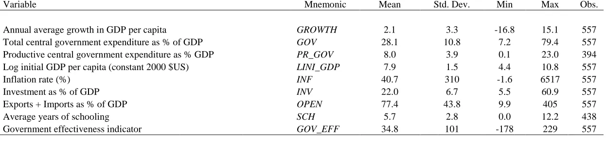
Table 1 provides summary statistics for the data and defines the variable

mnemonics used in the paper. A further breakdown of the sample according to five-year

averages is presented in Appendix A (Table A1).11 For our sample of countries, the

overall growth rate averaged 2.1 percent per annum. This masks a wide disparity across

countries and across time. While growth in the OECD countries averaged 2.6 percent per

annum, the corresponding rate in developing countries was 1.9 percent. Similarly, the

average size of government (measured as total expenditure to GDP) was 28.1 percent, but

the difference between high-income and low-income countries was stark, averaging 34.1

percent and 25.7 percent, respectively. Figure 1 plots the average government size against

average real GDP per capita growth for each country over the period 1970-2005. A

preliminary bivariate regression of these cross-sectional data suggests a positive—though

not statistically significant (p = .159)—relationship between the two variables of interest.

Model Specification and Estimation

Recall that according to the nonlinear hypothesis, the effect of government

expenditure on growth will vary depending on the size of government. We first test for

the presence of turning points or thresholds in the relationship between growth and

government size by applying the threshold regression model (Hansen, 1996, 1999, 2000).

The estimated threshold, provided it exists, is then interacted with government size.

The threshold regression model applied to a standard growth equation for country

i = 1, …, I and time period t = 1, …, T takes the following form:

it it

it it

it it

it X GOV I GOV GOV I GOV u

GROWTH 











and u_it 







where Xitrepresents the matrix of control variables, GOV denotes government spending

as a share of GDP, i is a country-specific fixed effect, t is a time fixed effect and it is a

normally distributed error term. I()is an indicator function which takes the value of one

when the condition inside parentheses is satisfied, and  is the threshold value to be

determined within the model. We define S()uˆ()'uˆ()as the residual sum of squares

of the model in (6) estimated for a threshold level The optimal threshold is then

ˆ argmin ().

 S

 (7)



ˆ

in one-unit increments.12

Having identified a potential threshold, it is important to determine whether the

threshold effect is statistically significant. From equation (6), testing for no threshold

effects is equivalent to testing the null hypothesis H0: 1= 2. However, since the null is

consistent with any arbitrary value of,the threshold cannot be identified using standard

methods of inference. Hansen (1996, 1999) suggests a bootstrap method to simulate the

asymptotic distribution of the likelihood ratio (LR) test of H0 based on:





1 0

0 S S (ˆ) /ˆ

LR   , (8)

where S0 denotes the residual sum of squares for the model with no threshold and ˆ2is

the estimated error variance in the presence of the threshold,



ˆ

distribution of LR0 is non-standard and strictly dominates the 2 distribution. The

12

distribution of LR0 depends in general on the moments of the sample, thus critical values

cannot be tabulated. However, Hansen shows that a bootstrap procedure attains the

first-order asymptotic distribution, so p-values constructed from the bootstrap are

asymptotically valid.13

It is also interesting to know how precisely the threshold has been estimated. The

asymptotic confidence interval for



ˆ





1() S() S(ˆ) /ˆ

LR   (9)

across the range of values for . We note that LR1() is a simple re-normalization of the

sequence of sum of squared residuals, S(), and takes the value of zero at



ˆ

shown that the LR1 statistic tends in distribution to the random variable with limiting

distribution Pr(



), 1 1 log( 2 )

(   

c gives the relevant 100% critical value.

Once the threshold has been identified and



ˆ

proceed to estimate equation (6) with standard econometric techniques.14 We rely mainly

on fixed effects estimation, controlling for both time-invariant individual country

characteristics and time fixed effects.15 In addition, we use dynamic panel system

generalized method of moments (Arellano & Bover, 1995; Blundell & Bond, 1998)

estimation to account for the possibility of reverse causality between growth and

13 _{The bootstrap procedure is outlined in Hansen (1999).} 14

Chan (1993) and Hansen (2000) show that the dependence of i on the threshold estimate is not of

first-order asymptotic importance, so inference on i can proceed as if the threshold estimate, ˆ , were the true value.

15 _{We also considered pooled OLS and two-way random effects models. Based on the log likelihood and}

government size under Wagner’s law (Easterly & Rebelo, 1993).16

The panel GMM

estimator has been used extensively (Beck & Levine, 2004; Johansson, 2010; Rioja &

Valev, 2004) to deal with problems arising from independent variables that are not

strictly exogenous. It has the advantage of using internal instruments, formulated from

lags of the endogenous variables themselves. Moreover, the system GMM estimator is

specifically designed to handle some of the problematic features of panel data such as

country-specific fixed effects, heteroskedasticity and autocorrelation within countries.17

Results

Threshold Existence

The threshold regression analysis indicates the existence of thresholds in the

relationship between growth and government size. Table 2 presents results of the

estimated location and significance levels of turning points in various sub-samples of the

data. The asymptotic p-values of the LR0statistic indicate that the null hypothesis of no

threshold effects can be rejected at least at the 5 percent significance level for all three

samples.

The overall threshold estimate for the full sample is indicated at 33 percent.

Figure 2 illustrates the distribution of observations according to government size and

16_{Wagner’s law states that there is a tendency for government expenditure to be higher at higher levels of}

per capita GDP. On the one hand, Wagner’s law may be less of a concern here, since it suggests an association between GDP growth and the growth rate, rather than the level, of government expenditure. However, to the extent that faster growing economies achieve a higher level of GDP, which has been shown to be associated with higher government spending, the possibility of a reverse relationship has to be considered.

17

GDP growth rates. Of the 557 observations in the full sample, 382 (69 percent) fall below

the estimated threshold. These observations represent 117 of the 136 countries in the full

sample. Figure 3 presents the likelihood ratio (LR1) statistics and corresponding

asymptotic confidence intervals for the threshold estimates.18 The large confidence

interval for the full sample (see panel a), casts doubt on the precision of this estimate. As

indicated above, the threshold location is likely to be affected by many things. One such

factor may be that the wide disparities among such a broad group of countries are

influencing the results (Bose, Holman, & Neanidis, 2007; Gregoriou & Ghosh, 2009;

Sheehey, 1993). Allowing for parametric heterogeneity between developed and

developing countries, we re-estimate the thresholds distinguishing between the two

country groups. This time the results again indicate an expenditure-to-GDP threshold at

33 percent for developing countries, which is highly significant at the one-percent level.19

More encouragingly, the narrow confidence intervals indicate greater precision of the

estimate. The second panel in Figure 3 illustrates that the 5 percent critical value crosses

the normalized LR1statistic over a narrow range. We can therefore say with 95 percent

confidence that the true threshold falls within the interval (29, 36).20

For developed countries, Table 2 indicates the presence of threshold effects at 26

percent, which is below the level of developing countries.21 One explanation for the

lower threshold result could be due to the composition of expenditures. We know that

18 _{The confidence interval of the threshold estimate of  consists of those values of government expenditure}

for which the likelihood ratio statistic is less than the critical value.

19 _{For the sample of developing countries, 316 out of 399 observations (79 percent) fall below the threshold}

( = 33); representing 98 out of 108 countries.

20 _{This is consistent with Varoudakis et al. (2007) who found an estimated threshold at 35 percent of total}

government spending for countries in Europe and Central Asia (ECA). It is notably larger than the average threshold estimates found by Sheehey (1993) and Karras (1996), who both employed consumption expenditure as their measure of government size.

21 _{For the sample of developed countries, 41 out of 158 observations (26 percent) fall below the estimated}

countries with bigger governments tend to allocate a larger share of total government

spending to social welfare and transfer payments (Gray, Lane, & Varoudakis, 2007). In

our estimation sample, developed countries allocate roughly 42 percent of total

expenditure to unproductive means, 22 compared to 30 percent in developing countries.

To the extent that this kind of spending has to be financed by tax revenues, then the lower

threshold corresponds to a lower optimal government size predicted by the nonlinear

hypothesis (Barro, 1990). We note that while the p-values indicate that the coefficients

for the regimes above and below the threshold are statistically different at least at the 5

percent level, the wide confidence intervals again restrict our conclusions about the

precision of this estimate.23

Threshold Effects

Total government spending.

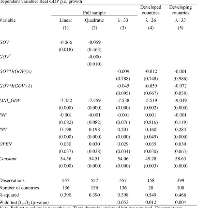
Table 3 reports the estimated effects of government spending on growth taking

into account the thresholds identified in the previous exercise. Results on threshold

effects for the full sample are presented in column 3, with the threshold specified at 33

percent. For comparison, we also include results for when the model is estimated without

accounting for nonlinearities (column 1) and when nonlinearities take a quadratic form

(column 2).24

22 _{Defined here as the sum of public spending on social security and welfare, recreation and economic}

services (Kneller et al., 1999).

23

We also tested for thresholds on various other sub-samples of the data based on geographical region (Karras, 1996) and income level. The threshold estimates, while varying slightly, are consistent with our main results, though less precisely estimated. More details are provided in Appendix A.

24

The main variable of interest is government size, GOV, as measured by total

government expenditure as a share of GDP. When entered linearly, the coefficient is

negative and statistically significant, p = .018. A one-percentage point increase in total

government expenditure reduces per capita real output growth by 0.07 of a percentage

point. Unsurprisingly, consistent with previous studies, the possibility of a nonlinear

effect is not captured by a quadratic specification. When a quadratic term on total

government spending is included, the model fails to find significance for either of the

fiscal variables.

The results for the nonlinear model with a threshold on government spending at

33 percent for the full sample, (column 3) suggest a weak nonlinear effect, but not of the

form expected from the Barro nonlinear hypothesis. Instead of displaying a positive

relationship with growth when government is small as would be predicted by the theory,

the effect of government spending below the threshold is negligible, being neither

statistically nor economically significant. Beyond the estimated threshold, the effect of

government spending is negative as expected, but only significant at the 10 percent level,

p = .095. The growth rate falls by 0.045 percentage points for every unit percentage point

increase in government size. Standard Wald tests confirm the two coefficients around the

threshold to be statistically different, p = .053.

Distinguishing between developed and developing countries gives similar results.

In developing countries (column 5), there is a significant negative effect only after the

threshold has been exceeded. For government size below 33 percent, the growth effect is

negligible. Wald tests show the two coefficients around the threshold to be statistically

also note significant differences around the estimated threshold of 26 percent. Above this

value, larger government size has a deleterious effect on growth but below the threshold,

there is no statistically significant effect even though the coefficient is negative.

These results are interesting as they seem to indicate the presence of nonlinearities

in the government size – growth relationship, but not in line with an expected inverted U-

shape. This would provide one explanation why previous studies using a quadratic

specification failed to capture the nonlinear effect. The quadratic model a priori restricts

the relationship between government size and long-run growth to a particular functional

form, which may or may not be in line with the true data-generating process. The

threshold model does not make this assumption but rather allows the data to suggest the

model specification. In this case, the data show that the nonlinear effect we investigate

does not display a smooth turning point around a defined optimum, but rather takes the

form of a kink where there is a distinct change in the slope. The threshold model is better

suited than the quadratic model to detect this kind of nonlinearity.

We note that the control variables have the expected signs and are all statistically

significant. The negative coefficient on initial GDP confirms the conditional convergence

hypothesis within a 5-year time span. Also as expected, increases in inflation reduce

growth, but the coefficient is small and weakly significant, p = .076. The coefficient on

the share of investment as a proportion of GDP is positive and highly significant, p <

.001. A one-percentage point increase in investment can stimulate long-run growth by 0.2

of a percentage point. This compares favorably with previous studies (Adam & Bevan,

2005; Bose et al., 2007). Finally, openness to trade (OPEN) also indicates a positive and

Endogeneity.

As previously discussed, one concern is that some of the explanatory variables,

including our main variable of interest, may not be strictly exogenous thus causing the

coefficients to be biased. We account for possible endogeneity issues by applying

dynamic panel GMM techniques to equation (6). Given observed differences between

developed and developing countries, we reestimate the full sample GMM equation

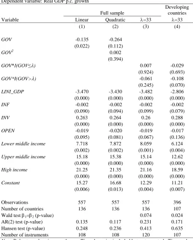
including income-class dummies for each country.25,26 The results for the GMM

regression on the full sample are presented in Table 4. For comparison, we provide the

results of the linear and quadratic models in the first two columns. We also include the

Arellano-Bond test for autocorrelation and the Hansen J test of over-identifying

restrictions.27 Both tests support the validity of the model in each regression.

Focusing on the threshold specification, column 3, we note that GMM estimation

indicates considerable change in the slope coefficients around the threshold value, but

neither side exhibits statistical significance. The negative coefficient above the threshold

is consistent with the FE model, but under GMM the standard errors are larger.

Interestingly, for government spending below the threshold, the GMM estimation returns

a positive coefficient. Not surprisingly, when the model is estimated only for developing

countries, column 4, results are more in line with the fixed effects specification, with a

weakly significant negative coefficient above the threshold, (p = .070), and no

statistically significant effect below. This helps to reassure us that the main results are not

25 _{Dynamic panel GMM does not perform well in small samples with many regressors making it unsuitable}

for estimation of the developed country sub-sample which has only 158 observations (Roodman, 2009b).

26

We use the World Bank country classification which groups countries into low-income, lower-middle income, upper-middle income and high-income country groups.

27

merely an artifact of endogeneity biases. While the coefficients on the control variables

are of different magnitudes, the signs are largely as expected with different levels of

significance. The only exception is OPEN which has an unexpected negative sign. In

addition, as in the fixed effects model, when nonlinearities are ignored, the coefficient on

the government size variable is strongly negative and significant, p = .022. However,

under GMM it is about twice the magnitude.

Productive government spending.

Even though the results show that the effect of government spending below the

threshold is statistically insignificant, we would have expected the coefficient to at least

display a positive sign. One possible explanation for this puzzle is in noting that the

theory makes a distinction between productive and unproductive public spending and it is

the productive portion which is growth-enhancing, while the unproductive share is

theorized to have a negative effect. In analyzing the total spending, we are indeed

confounding the two effects, which may have offsetting influences. We therefore try to

isolate what may be considered as productive elements of government spending. Using

the functional classification of the GFS, we define productive government spending,

PR_GOV, as the sum of expenditure on education, health, housing, transport and

communication, relative to GDP.28 Similar definitions have been used by Adam and

Bevan (2005), Kneller et al. (1999) and Park (2006). We note that more detailed

information is required to construct this variable and many missing observations result in

a smaller sample size, reducing the number of observations from 557 to 394 in some

specifications.

28 _{Several empirical studies have shown public spending in these particular areas to be positively associated}

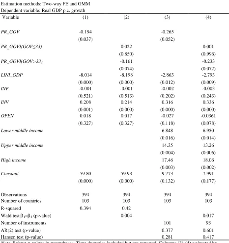
The regression results focusing on productive government spending are presented

in Table 5. In column 1, we estimate a linear specification without controlling for total

government size. The results are similar to the comparable case using total spending. In

column 2 we re-estimate the baseline threshold model (equation 6) replacing total

government spending with productive government spending, but maintaining total size as

the variable on which the threshold is based.29 Now, in line with expectations, the

coefficients on the fiscal variables change sign around the threshold value. Below the

threshold, when total government spending is less than 33 percent, the coefficient on

productive government spending is positive, though still not statistically significant.

When the total size of government increases beyond the threshold value further increases

in productive spending have a negative significant effect on growth, so that even

expenditure on productive activities does not translate into long-run growth. In columns 3

and 4, we re-estimate the productive spending models using dynamic GMM to account

for endogeneity. We find that the results are consistent with the fixed effects

specification.

We also estimated the model separately for developed and developing countries

(Table A3 in Appendix A). When focusing on productive expenditure, the government

size threshold value for developed countries was higher at 32 percent while that for

developing countries remained the same at 33 percent. A statistically significant change

in slope was evident around the threshold value in either case, but only the developing

countries displayed a change in sign.

29

The model estimated was

it it

it it

it it

it X PR GOV I GOV PR GOV I GOV u

GROWTH ₀ ₁ _  ( )₂ _  ( ) . A new threshold search revealed ˆ at 33 percent, consistent with the original sample. Testing the null hypothesis for the difference in slopes gives an LR0 statistic of 10.968 which is significant at the 1 percent level.

Sensitivity Analysis

We test the robustness of the main results under various alternative specifications

and sub-samples. The tests give results generally in line with the main findings reported

in Tables 3-5, with some caveats.

We first examine how sensitive the results are to alternative combinations of

covariates in the control vector. Alternatively excluding INF, INV and OPEN from the

main specification in equation (6), we find that both the threshold value and the

qualitative effects around the threshold remain consistent with the primary results (see

columns 1-3 in Table A4). However, when additional controls are incorporated the results

vary. Including average years of schooling to control for the level of human capital

(Barro & Sala-i-Martin, 1995; Levine & Renelt, 1992) does not support the existence of a

threshold as



ˆ

specification of the fiscal variable is more appropriate.

A number of studies have explored the importance of the quality of institutions in

the development process (Acemoglu, Johnson, Robinson, & Thaicharoen, 2003; Knack &

Keefer, 1995). Following on Varoudakis et al. (2007) who suggest that the quality of

government may be an additional source of nonlinearity in the government size – growth

relationship, we split the sample in two according to the countries which display high

levels of effectiveness in government and those that are less effective.30 Reestimating the

threshold regression on either subsample, we find evidence of thresholds at 30 and 33

percent, respectively. Further, it would appear that the nonlinear effect of government

30

spending is more dominant in countries with low government effectiveness. On the other

hand, highly effective governments seem to be able to offset some of the negative impact

of large size. These results for a broad sample of countries are in line with Varoudakis et

al. who find similar effects for the transitional economies.

The second set of robustness checks explores how sensitive the main findings are

to diverse subsamples of the data. We divide developing countries into four geographical

regions (Africa, Latin America, South and East Asia and Europe and Central Asia

[ECA]).31 The estimated threshold values varied between 33 and 41 percent with

noticeable variations in the coefficients on either side of the threshold (Table A5).

Notably, for developing countries in Asia and the ECA, government expenditure for

countries below the threshold had a positive and statistically significant effect. Findings

from income-based subgroups also showed variations around the threshold consistent

with the main results (Table A6).

In addition, we varied the sample on the basis of time to check for possible

sample selection bias introduced by using an unbalanced panel. As we mentioned, data in

the earliest years are more prone to missing observations, particularly from the

developing countries. As a test we exclude observations from the first decade of our

sample, limiting the estimation sample period to 1981-2005. This reduces the number of

observations to 447, even though cross-sectionally country coverage is almost unchanged

(see column 1 of Table A7). Fixed effects estimation of the threshold model suggests

there may be sample selection bias. While the coefficient on government spending above

the threshold remains negative and of similar magnitude, the standard errors are larger

31 _{Karras (1996) finds that the optimal government size varies across different geographical regions and}

causing it to lose statistical significance. Likewise, the coefficient on government

spending above the threshold is positive, though as in the main analysis, not significant.

Notably, the coefficients on the control variables remain largely unchanged, except for

openness, which loses significance. Similar effects are found for further variations in the

sample period. While sample selection bias may be present in the full panel, the overall

results prove to be qualitatively robust over various other subsample specifications.

Conclusion

This paper reexamined the relationship between government spending and

long-run economic growth. In light of prevailing theory, which predicts a nonlinear

relationship between tax-financed government expenditure and output growth, and in

view of inconsistent results from various empirical studies on the subject, we sought to

evaluate the Barro hypothesis by explicitly testing for the existence of thresholds in the

government size and growth relationship. We applied threshold regression methods

developed by Hansen (2000) to a panel of 136 developed and developing countries over

the period 1971-2005. Using a comprehensive measure of government spending, we were

able to isolate productive elements in various regression specifications. Furthermore, we

addressed potential simultaneity biases in the government size – growth relationship by

also using GMM dynamic estimation techniques.

We find evidence to support a nonlinear effect, but not of the form suggested by

Barro’s nonlinear hypothesis. For total government spending above a critical threshold,

we find a weakly significant negative effect on growth. However, this effect is negligible

statistically significant—coefficient when productive government spending is

distinguished from the total. We also find evidence to suggest that the level of economic

development and the quality of government present additional sources of potential

nonlinearities. When we analyze developed and developing countries separately, the

threshold location is lower for developed countries at 26-32 percent. High quality

governance mitigated some of the negative effects so that nonlinearities were more

pronounced in countries with less effective governments. Finally, we showed that our

results were not driven by endogeneity issues and were generally qualitatively robust to

various specifications and estimation techniques.

The findings of this paper have significant public policy implications as they offer

some insight to the policy debate about the optimal size of government, and how this

varies according to the level of economic development of a country. Indeed, as indicative

from the sample of 28 developed countries, almost three-quarters of which have a

government size exceeding 30 percent of GDP as of 2001-2005, the concern about large

governments is not misplaced. Ever-expanding governments will have negative effects on

long-run growth in these economies. Fortunately, the evidence also shows that

improvements to the quality of government can dampen these negative effects. On

another note, the negligible growth effects of government spending below the threshold

imply serious offsetting influences between productive and unproductive expenditure,

which mitigate the potential benefits from increased public spending. This points to a

necessary restructuring of fiscal budgets towards spending in areas proven to be

growth-enhancing. Creating the ―fiscal space‖ to provide productive capital that will engender

Of course, the optimal composition and financing of government expenditures

matters. While there has been some work on how these aspects of government spending

affect its impact on growth, much more work needs to be done in order to arrive at clear,

ESSAY 2

FINANCING PRODUCTIVE GOVERNMENT EXPENDITURES:

THE IMPORTANCE OF INITIAL FISCAL CONDITIONS

Introduction

Endogenous growth theory provides a foundation for the role of productive

government spending in fostering long-term economic growth. Government provision of

public capital to the production process contributes to growth directly by adding to the

existing capital stock, as well as indirectly by raising the marginal productivity of

privately supplied factors of production (Barro, 1990; Tanzi & Zee, 1997). While what

exactly constitutes productive government spending in practice is debatable,32 there

seems to be consensus that public investment in basic physical infrastructure such as

roads, transportation and communication is growth-enhancing. Spending in these areas

has been shown empirically to have a positive impact on aggregate production and is

considered crucial for long-term growth and development.33 Likewise, a broader concept

of capital to include both physical and human capital (e.g., Garcia-Mila & McGuire,

1992; Mera, 1973) has led to studies which demonstrate that public spending to augment

the stock and quality of human capital, such as public investment in education and

32 _{The productivity of public spending may vary according to, inter alia, the potential returns on the}

specific project being funded, how efficiently public funds are used (which may depend on the institutional quality of the government), and the extent of the imbalance in the relative shares between public and private capital, giving rise to diminishing marginal returns.

33 _{For a general review of the literature see Tanzi and Zee (1997). Early empirical work by Aschauer (1989)}

healthcare, also has significant growth effects in the long-run.34 More recently, it has

been shown that complementarities between various types of public capital can generate

additional externalities which increase growth (Agénor & Moreno-Dodson, 2006; Agénor

& Neanidis, 2006).

Given the potential for productive government expenditure to raise long-term

economic growth rates, it is of major concern that in many countries which undergo fiscal

adjustments, the first budget items typically slashed are those categories most associated

with growth. Latin America has been a particularly extreme case with a history of debt

defaults and high debt-to-output ratios. In the 1980s and 1990s, the region engaged in a

wave of fiscal adjustment initiatives aimed at scaling back government activity,

increasing revenue generation and bringing debt to sustainable levels (Calderòn &

Servèn, 2004; Easterly, Irwin, & Servèn, 2008). Declines in fiscal deficits seemed to be

largely driven by cuts in public investment. It is estimated that in the five largest

economies, infrastructure investment cuts alone contributed at least half of the total fiscal

adjustments (Calderòn, Easterly, & Servèn, 2003a,b).

The fallout in productive government expenditure is particularly deleterious in

developing countries in general because the state plays a more active role in production,

with public capital representing a much larger share of the aggregate capital stock than in

34

industrial countries (Agénor & Montiel, 2008). In Latin America, cuts in public

infrastructure investment were not fully offset by private sector investment. As a result,

total infrastructure investment fell, reaching well below the level that would be required

for sustained growth in the region (Calderòn & Servèn, 2010; Fay & Morrison, 2005).

Furthermore, with the phenomenally high degree of inequality in Latin America,

shortfalls in public provision of education and healthcare services would have a

disproportionate impact on the poor, perpetuating a cycle of low education, low skill and

low incomes for a significant fraction of the population, thus severely limiting human

capital accumulation (Agénor, 2004).

It is then clear that policymakers in developing countries run the risk of stagnating

their economies over the long run if the appropriate level and composition of public

investment is not established and maintained. Of course, a major challenge facing

governments is how to finance such expenditures given binding fiscal constraints.

Moreover, it has been shown that diverse types of government expenditure may have

conflicting effects on growth given different sources of financing. Income taxes tend to

be distortionary creating disincentives to saving and investment, while deficit financing

may crowd out private investment (Agénor, 2004; Kneller et al., 1999). It is therefore

important to know how government spending can be most efficiently allocated and

financed to bring about optimal growth results, particularly in the context of already high

tax rates, large fiscal deficits, and growing debt stocks.

This chapter develops a dynamic macroeconomic model for a representative

closed economy to explore how variations in the composition and financing of

to analyze how public investment spending funded by taxes (income or consumption) or

by borrowing affects long-term output growth. We also examine the effect of varying the

composition of public expenditure, shifting between consumption and investment

spending, or re-allocating between different types of public investment. In addition, we

explore how heterogeneous fiscal conditions affect the implications for growth.

Specifically, we use alternative parameterizations of the model to simulate extreme initial

fiscal conditions such as high average tax rates, debt stock ratios and government

consumption spending.

The model is calibrated to reflect economic conditions in the seven largest Latin

American economies during the period 1990 to 2008. The Latin American countries

provide a suitable testing ground for the implications of the model given their debt

history and diverse fiscal adjustment experiences. We find that, when tax rates are not

already high, funding public investment by raising taxes may increase long-run growth. If

existing tax rates are high, then public investment is only growth-enhancing if funded by

restructuring the composition of public spending. Interestingly, using debt to finance new

public investment compromises long-run growth, regardless of the initial fiscal condition.

The paper contributes to the existing literature in a number of ways. First, we take

into account that government expenditure is not homogeneous and spending in different

sectors will have diverse productivities (Feltenstein & Ha, 1995). Thus, we move beyond

the standard practice of broadly categorizing government spending merely as

―productive‖ or ―unproductive‖ and explicitly recognize the heterogeneity within

productive government expenditure itself. To do this, we develop a two-sector