A Study of the Lhires III Spectrograph on the Hard Labor Creek Observatory 20 inch Telescope

ScholarWorks @ Georgia State University

ScholarWorks @ Georgia State University

Mathematics Theses Department of Mathematics and Statistics

Spring 4-20-2011

Modified Profile Likelihood Approach for Certain Intraclass

Modified Profile Likelihood Approach for Certain Intraclass

Correlation Coefficient

Correlation Coefficient

Huayu Liu

Follow this and additional works at: https://scholarworks.gsu.edu/math_theses

Recommended Citation Recommended Citation

Liu, Huayu, "Modified Profile Likelihood Approach for Certain Intraclass Correlation Coefficient." Thesis, Georgia State University, 2011.

https://scholarworks.gsu.edu/math_theses/96

by

HUAYU LIU

Under the Direction of Dr. YUANHUI XIAO

ABSTRACT

In this paper we consider the problem of constructing confidence intervals and lower

bounds for the intraclass correlation coefficient in an interrater reliability study where the

raters are randomly selected from a population of raters.The likelihood function of the

inter-rater reliability is derived and simplified, and the profile likelihood based approach is readily

available for computing the confidence intervals of the interrater reliability. Unfortunately,

the confidence intervals computed by using the profile likelihood function are in general too

narrow to have the desired coverage probabilities. From the point view of practice, a

con-servative approach, if is at least as precise as any existing method, is preferred since it gives

the correct results with a probability higher than claimed. Under this rationale, we propose

the so-called modified profile likelihoodapproach in this paper. Simulation study shows that,

the proposed method in general has better performance than currently used methods.

CORRELATION COEFFICIENTS

by

HUAYU LIU

A Dissertation Submitted in Partial Fulfillment of the Requirements for the Degree of

Master of Science

in the College of Arts and Sciences

Georgia State University

CORRELATION COEFFICIENTSK

by

HUAYU LIU

Committee Chair: Dr. Yuanhui Xiao

Committee: Dr. Yichuan Zhao

Dr. Xu Zhang

Electronic Version Approved:

Office of Graduate Studies

College of Arts and Sciences

Georgia State University

ACKNOWLEDGEMENTS

Foremost, I would like to give most sincere thanks to my advisor Dr. Yuanhui Xiao for his

constant support, abundant help and invaluable advice for my research and study in

Geor-gia State University. With patience and motivation, he has given me timely guidance in the

critical stages of my research and especially towards the completion of this thesis.

Secondly, I am thankful for the fact that Dr. Zhao and Dr. Zhang would like to be my

the-sis committee members. I appreciate their time to read my thethe-sis and give me salient advice.

Last but most importantly, I would like to thank my husband Shenjia Zhang for his caring

love and selfless support, which makes my life, study and research in Georgia State university

TABLE OF CONTENTS

ACKNOWLEDGEMENTS . . . iv

LIST OF TABLES . . . vi

Chapter 1 INTRODUCTION . . . 1

Chapter 2 THE GENERAL VARIABLE APPROACH . . . 5

Chapter 3 LIKELIHOOD BASED INTERVAL ESTIMATION FOR ρ 7 Chapter 4 A SIMULATION STUDY . . . 12

Chapter 5 EXAMPLES . . . 20

Chapter 6 DISCUSSIONS AND FUTURE WORKS . . . 22

LIST OF TABLES

Table 1.1 Analysis of variance for the results of an interrater reliability study 3

Table 3.1 Estimates of κm for two-sided 90% confidence intervals and one-sided

95% confidence lower bounds ofρ(based on 20,000 simulated samples) 11

Table 4.1 Empirical probabilities (×1000) and average lengths of approximate 90% confidence intervals for ρ (based on 20,000 simulations). For the

PL method,κ = 0. . . 13

Table 4.2 Empirical probabilities (×1000) and average lengths of approximate 90% confidence intervals forρ (based on 20,000 simulations) as well as

the estimates ofκ. For the PL method,κ = ˆκopt. . . 15

Table 4.3 Empirical probabilities (×1000) and average lengths of approximate 90% confidence intervals for ρ (based on 20,000 simulations). For the

MPL method, κm equals to the estimates corresponding to δU = 16 in

Table 3.1. . . 16

Table 4.4 Empirical probabilities (×1000) and “average lengths” of approximate 95% confidence lower bounds for ρ(based on 20,000 simulations). For

the PL method, κ= 0. . . 17

Table 4.5 Empirical probabilities (×1000) and average lengths of approximate 95% confidence lower bounds for ρ (based on 20,000 simulations) as

Table 4.6 Empirical probabilities (×1000) and average lengths of approximate 90% confidence lower bounds for ρ(based on 20,000 simulations). For

the MPL method, κm equals to the values corresponding to δU = 16

Chapter 1

INTRODUCTION

The intraclass correlation coefficient,which defined by Harggard [?] as ”the measure

of relative homogeneity of the score within classes in relation to the total variance”, has

been widely adapted in behavior and biomedical science. Its first application dates back

to Pearson in his study of measuring family resemblance of height of brothers. There are

basically two major objects with which Intraclass correlation coefficient is used: to measure

the sameness for unit in the same group, or reliability test, where measurement error is

introduced by rates.

In this paper we consider the interrater reliability study in which each of R raters measures

each of S subjects. Suppose each of the random sample of R raters in the reliability study

rates each of the corresponding random sample ofS subjects independently, the rating score

Yij of the ith rater on the jth subject may be represented as

Yij =µ+ri+sj +eij, (i= 1,2, . . . , R; j = 1,2, . . . , S), (1.1)

where µis the overall population mean of the measurements, ri reflects the effect of the ith

rater,sj characterizes the effect of thejth subject andeij is the measurement error associated

with this rating. The random variablesri,sj andeij are assumed to be mutually independent

and normally distributed with zero mean 0 and variances σ2

r, σ2s and σ2e, respectively. The

variance σ2 of Yij is

σ2 ≡var(Yij) = σ2r+σ 2 s +σ

2

and the covariance between two measurements taken by the ith andi0th raters on the same

subject j is

cov(Yij, Yi0_j) =σ_s2. (1.3)

It follows that the appropriate intraclass correlation coefficient to measure interrater

relia-bility is

ρ= σ

2 s σ2 ≡

σ2 s σ2

s +σ2r+σe2

. (1.4)

The value ofρrepresents the proportion of total variability on observed scores accounted for

by the subject-to-subject variability in the true but unobservable scores. To emphasize this

fact, it is also denoted by ρs. Throughout this paper, ρ and ρs are used interchangeably.

(Similarly, the quantity ρr given by the following equation

ρr = σ_r2 σ2 ≡

σ_r2 σ2

s +σr2+σ2e

(1.5)

is the proportion of total variability on observed scores accounted for by the rater-to-rater

variability in the true score. The ratio of rater-to-error variability is defined as

δ= σ

2 r σ2 e

≡ ρr

1−ρs−ρr

, (1.6)

which is also an important parameter of the model (1.1). Obviously,ρs>0, ρr >0, ρs+ρr<

1.)

As the assessment of reliability of measurement is of great importance in medical study,

where measurement error may have serious unwanted consequence, considerable amount of

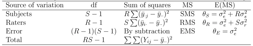
research has been done for ρ. See [7], [1], [14], [2] and [10], etc. Table 1.1 presents the

analysis of variance layout corresponding to the two-way random effects model (1.1). From

this table, the unbiased estimators of the three components of variances σ2_s, σ2_r, σ_e2 are

s2

Table 1.1. Analysis of variance for the results of an interrater reliability study

Source of variation df Sum of squares MS E(MS)

Subjects S−1 RP

(¯y·j−y¯··)2 SMS θS =σe2+Rσs2

Raters R−1 SP

(¯yi·−y¯··)2 RMS θR=σ2e+Sσ2r

Error (R−1)(S−1) By subtraction EMS θE =σe2

Total RS−1 P P

(Yij −y¯··)2

is then estimated by

ˆ

ρ= s

2 s s2

s+s2r+s2e

= S×(SM S−EM S)

S×SM S+R×RM S+ (RS−R−S)×EM S (1.7)

This approach was proposed by Rajaratnam [7] and Rajaratnam[1]. The method is in

general biased and the resulting estimates may be negative. Fortunately, the bias decreases

as both R and S increase.

Fleiss [4] developed an approach for interval estimation ofρbased on Satterthwaite’s[8]

two-moment approximation. This method has been widely used, but it understates the

coverage probabilities substantially in certain cases. The problem has been noticed by Zou

et al.[14], so they proposed a three-moment approximation and a four-moment approximation

by using the Pearson system of distribution under the rationale that a better approximation

may be achieved by using higher moments. In general, their higher-moment approaches

produce confidence intervals that are more conservative and satisfactory than those produced

by two-moment approaches.

However, Cappelleri [2] found that, in certain situations, (for example, when there are

only three raters, or the ratio of rater-to-error variability is relatively high.), the

higher-moment approaches tend to understate the coverage probabilities. Therefore, they proposed

a modified large-sample approach (MLS), which produces either correct or conservative

con-fidence intervals with more precise (narrower) widths than those generated by the

By using generalized variables (Section 2), Tian et al.[10] proposed an approach for

estimating the two-sided confidence intervals or one-side confidence lower bounds of ρ. The

generalized variable method (GV) in general has a behavior similar to that of the MLS.

In certain situations, (e.g., when the ratio of rater-to-error variability is about 0.5), the

coverage probabilities of one-sided confidence intervals produced by the GV method (i.e., the

method using generalized variables) are marginally more conservative than that produced by

MLS. Based on simulation studies, the GV method has the best overall performance among

existing methods.

It seems that no existing method for estimating the confidence intervals ofρ is based on

likelihood approach. However, through a series of algebraic operations, we find found that the

likelihood function of (1.1) has an explicit expression which is extremely simple (Appendix),

so we will develop methods for constructing confidence intervals and computing the lower

bounds for ρ based on profile likelihood approach. In general, the confidence intervals of ρ

produced by the traditional profile-likelihood approach are too narrow to have the desired

coverage probabilities, so a remedy is necessary, resulting in the modified profile likelihood

(MPL) approach proposed in this paper. The detail is described in Section 3. The proposed

approach is assessed by a Monte-Carlo simulation study, where its performance is compared

with that of the GV approach in terms of coverage probabilities and average lengths of the

respective confidence intervals. The GV method is chosen for comparison purpose not only

because it is one of the most competent methods, but also easy to implement. The results

of the simulation study are presented and analyzed in Section 4. The performance of the

modified profile likelihood approach will be furtherly discussed in the last section. Before we

introduce the proposed approach, we will give a short description of the generalized variable

Chapter 2

THE GENERAL VARIABLE APPROACH

Suppose that X = (X1, X2, . . . , Xn) constitute a random sample from a distribution

which depends on the parameters β = (θ,ν), where θ is of interest and ν is a vector of

nuisance parameters. Letxis be an observed value ofX, a generalized variableR(X;x, θ,ν)

for interval estimation of θ has the following two properties:

1. R(X;x, θ,ν) has a distribution free of unknown parameters;

2. R(x;x, θ,ν) =θ.

See Weerahandi [12]. To construct confidence intervals for the intraclass correlation

coeffi-cientρ, [10] proposed the following generalized variable

Rρ =

sms θS

SMS−ems θE

EMS

sms θS

SMS + (R/S)rms θR

RMS + [R−1−(R/S)]ems θE

EMS

= sms

S−1

QS −ems

(R−1)(S−1) QE

smsS_Q−1

S + (R/S)rms

R−1

QR + [R−1−(R/S)]ems

(R−1)(S−1) QE

,

(2.1)

whereQS = (S−1)SMS/θS,QR= (R−1)RMS/θR, andQE = (R−1)(S−1)EMS/θE. (Note

that, hereX = (SMS,RMS,EMS) andx= (sms,rms,ems).) The random variablesQS, QR

and QE are independent and distributed as χ2S−1, χ 2

R−1, and χ 2

(R−1)(S−1), respectively.

To construct a confidence interval for ρ, first we simulate a large number of triples

(QS, QR, QE) of random numbers from the chi-square distributions with degrees of freedoms

S−1, S−1 and (R−1)(S −1), respectively. Then the same number of values of Rρ are

computed via (2.1). The sample quantiles (denoted by Rρ,γ, where 0 < γ < 1) of those

confidence interval is computed as (Rρ,α/2, Rρ,1−α/2) and the one-sided 100(1−α)% lower

Chapter 3

LIKELIHOOD BASED INTERVAL ESTIMATION FOR ρ

It follows from (28), (29), (30), (31) and (56) in the Appendix that the negative twice

logarithm of the likelihood function l of ρ (= ρs) andρr, is given by

−2l=c0+ ln[1 + (R−1)ρs+ (S−1)ρr] (3.1)

+ (S−1) ln[1 + (R−1)ρs−ρr] (3.2)

+ (R−1) ln[1−ρs+ (S−1)ρr] (3.3)

+ (R−1)(S−1) ln[1−ρs−ρr] (3.4)

+RSln

(S−1)SMS 1−ρr+ (R−1)ρs

+ (R−1)RMS

1 + (S−1)ρr−ρs

+ (R−1)(S−1)EMS 1−ρs−ρr

, (3.5)

wherec0 is a constant free from the data and the parameters. Interestingly, the log-likelihood

function is a “function” of the ANOVA layout in Table 1.1. The profile log likelihood function

for ρ (≡ρs) is

l†(ρ;y) = max{l(ρ, ρr;y) : 0 < ρr <1−ρ}. (3.6)

Supposel†(ρ;y) achieves its maximum at ˆρ, then ˆρ is also the maximum likelihood estimate

(MLE) of ρ. An approximate two-side 100(1−α)% (0 < α <1) confidence interval for ρ is obtained as

ρ: 2l†( ˆρ;y)−2l†(ρ;y)≤(1 +κ)χ2_1,1−α , (3.7)

and an approximate one-side 100(1−α)% lower bound is computed as the smaller root of the following equation for ρ,

where κis an appropriately chosen constant in (3.7) and (3.8), respectively. The confidence

bounds in (3.7) and (3.8) are actually computed by a one-dimensional root-finding routine

nesting a one-dimensional optimization method.

According to the traditional likelihood theory, the constant κ is set to be zero, but in

our case the coverage probabilities will be in general understated, as shown in the simulation

study in Section 4. Ideally, we wish to choose the value of κ that would result in correct

confidence intervals. This value ofκ is termed the “correct value” ofκ and denoted byκcorr.

Accordingly to the likelihood theory, the correct value κcorr approaches to zero as both the

numbers of raters and subjects increase.

The correct valueκcorr depends on ρs,ρr, R (the number of raters) and S (the number

of subjects). a trackable expression is hardly available for it, thus it is infeasible to useκcorr

in practice. If we use a value of κ that is larger than κcorr, then the resulting confidence

intervals will be conservative in the sense that the coverage probability is higher than 1−α. The cost of achieving higher coverage probabilities is the loss of accuracy since the confidence

intervals would become wider. Suppose (ρL, ρU) and (δL, δU) are known ranges of ρ and δ,

respectively, then for fixed values of R and S, letting κ equal to the value of

κm = max{κcorr ≡κcorr(ρ, δ) : ρL≤ρ≤ρU; δL ≤δ≤δU}, (3.9)

would minimize the loss of accuracy. If we use κm or an estimate of κm in (3.7) or (3.8), the

resulting method will be called as modified profile likelihood (MPL) approach. Suppose we

know the modified profile likelihood would produce confidence intervals which are in average

shorter than those by a widely used method, then we may put this approach in our tool-box

for practical use since it is not only more precise than the widely used approach, but also

captures the true parameter value with a probability higher than claimed. That the modified

profile likelihood approach is more accurate than existing methods, which is illustrated by

In real life, we can hardly expect a value of ρ that is lower than 0.6, so we can set the

lower bound ofρto beρL= 0.6. As for the upper boundρU ofρ, we can safely setρU = 0.98

in most cases. Several authors used the values 0.5, 1.0, 4.0 of δ in their simulation study.

Conservatively, in most cases we may setδL = 0.5 and δU = 16.

Simulation study (not presented, but the reader is referred to Table 4.2 and Table 4.5)

shows that, roughly κcorr is an increasing function of δ for fixed value of ρ but a decreasing

function of ρ for fixed value of δ. Thus, an estimate of κm can be obtained by using a grid

search as follows. First we choose two positive values d and r, and define the grid points

(ρi, δj) as

ρi =ρL+ (i−1)d, i= 1,2, . . . , n1 (≤

ρU−ρL d + 1),

δj =rj, k1 ≤j ≤k2 ( so δL =rk1, and δU =rk2).

(3.10)

Then a reasonable estimate for κm is

ˆ

κm = max{κcorr(ρi, δj) : 1≤i≤n1; k1 ≤j ≤k2}. (3.11)

Usually we use d= 0.1 or d= 0.05 andr = 2, k1 =−1, k2 = 4 for computing ˆκm.

For known parameter values ofρandδ, the optimal valueκcorr can be obtained through a

grid search incorporated with Monte-Carlo simulation. Suppose we want to search for κcorr

in the interval [κL, κU] of κ, we can simulate the coverage probability at the grid points

κi = κL + (i−1)∗ dκ, i = 1,2, . . .;i ≤ (κU −κL)/dκ, where dκ > 0 is the increment,

and select the smallest κi for which the simulated coverage probability is not less than the

expected coverage probability. Here are the steps:

1. Choose κL, κU and dκ, and compute the value for each κi.

2. Generate a sample according to (1.1) by using given parameter values.

3. Compute the upper confidence bound ˆρU,0 of (3.7) and/or the lower confidence bound

ˆ

4. For i = 2, . . ., search for the upper confidence bound ˆρU,i of (3.7) in the interval

[ ˆρU,i−1,1] forκi, and/or the lower confidence bound ˆρL,i of (3.7) or (3.8) in the interval

[0,ρˆL,i−1] for κi.

5. For each κi, check if the corresponding confidence interval includes the true value ofρ.

6. Repeat the steps 2 - 5 m times, where m is a large number (say 10, 000 or 20,000).

For eachκi, record the number of confidence intervals that include the true value ofρ.

7. Finally, compute the proportion of confidence intervals that conclude the true value of

ρ for each κi (which is the simulated coverage probability), and select the smallest κi

for which the simulated coverage probability is at least 1−α as an approximation to κcorr.

With probability one, the value of κ thus obtained is not less than the actual value ofκcorr.

Usually, we may set κL =−0.20, κU = 0.8 and dκ = 0.05.

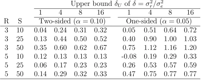
Table 3.1 presents the estimated values ofκm for various numbers of raters and subjects

by using the above methods with the following settings: m = 20,000; ρL = 0.6, ρU =

0.9, d = 0.1; r = 2, k1 = −1 (so δL = 0.5), k2 = 4 (so δU is equal to the values in the

table); dκ = 0.01; α = 0.10, κL = 0.0, κU = 0.80 for two-sided confidence intervals and

Table 3.1. Estimates of κm for two-sided 90% confidence intervals and one-sided 95%

confidence lower bounds of ρ (based on 20,000 simulated samples) Upper bound δU of δ=σ2r/σe2

1 4 8 16 1 4 8 16

R S Two-sided (α= 0.10) One-sided (α = 0.05)

3 10 0.04 0.24 0.31 0.32 0.05 0.51 0.64 0.72

3 25 0.13 0.44 0.50 0.52 0.40 0.90 1.00 1.03

3 50 0.35 0.60 0.62 0.67 0.75 1.12 1.16 1.20

5 10 0.12 0.13 0.13 0.13 -0.08 0.19 0.29 0.33

5 25 0.06 0.17 0.23 0.23 0.26 0.53 0.57 0.59

Chapter 4

A SIMULATION STUDY

The main purpose of this Monte-Carlo simulation study is to compare the performance

of the modified profile likelihood approach (MPL) with that of the GV approach described

in [10], so the parameter settings in [10] were used here. That is, the number of raters were

R = 3 and 5; the number of subjects were S = 10, 25 and 50; the value of ratio of

ratio-to-error variability σ2

r/σe2 were 0.5, 1.0, 4.0; the value of ρ were 0.6, 0.75, 0.90. For each

parameter setting, 20,000 random samples were generated. For the GV approach, 10,000

values of Rρ’s were created for each of the 20,000 random samples.

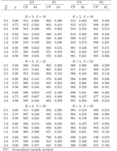
Tables 4.1 - 4.3 present the results about two-sided confidence intervals forρ produced

by the GV approach and the PL approach with different values of κ. The results for the

PL method with κ = 0 are presented in Table 4.1, where we can see that, in all cases the

average length of the confidence intervals produced by the PL approach is significantly shorter

than that by the GV method. Unfortunately, the PL approach consistently understates the

coverage probabilities. This phenomenon is obvious especially when the number of raters is

only three, or the number of subjects is large (S = 50), or the value of δ is high.

After a careful examination of the results in Table 4.1 we find that, the confidence

intervals produced by the PL approach with κ= 0 is “unnecessarily” narrow. For example,

when R= 3, S = 50, δ= 4.0 and ρ= 0.6, (This is the worst case for the PL method in the

sense that the coverage probability is extremely low, only 79.6%), the average length of the

confidence intervals from the PL approach is 0.420, while that from the GV method is 0.604.

This fact gives us the confidence to increase the value ofκfor achieving the desired coverage

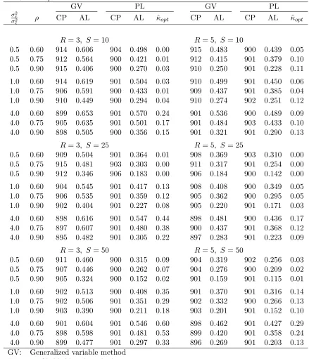
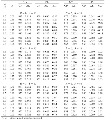
probabilities with comparable precision. Table 4.2 has the results for the PL approach with

Table 4.1. Empirical probabilities (×1000) and average lengths of approximate 90% confidence intervals for ρ (based on 20,000 simulations). For the PL method, κ= 0.

GV PL GV PL

σ2

r

σ2

e ρ CP AL CP AL CP AL CP AL

R= 3, S= 10 R = 5, S= 10

0.5 0.60 914 0.606 902 0.498 915 0.483 891 0.428

0.5 0.75 912 0.564 902 0.419 912 0.415 889 0.361

0.5 0.90 915 0.406 895 0.263 910 0.250 881 0.213

1.0 0.60 914 0.619 898 0.497 910 0.499 895 0.438

1.0 0.75 906 0.591 898 0.430 909 0.437 887 0.376

1.0 0.90 910 0.449 892 0.286 910 0.274 886 0.231

4.0 0.60 899 0.653 863 0.516 901 0.536 887 0.471

4.0 0.75 905 0.635 871 0.459 901 0.484 887 0.412

4.0 0.90 898 0.505 878 0.322 901 0.321 885 0.266

R= 3, S= 25 R = 5, S= 25

0.5 0.60 909 0.504 902 0.362 908 0.369 900 0.309

0.5 0.75 915 0.481 901 0.301 911 0.317 900 0.255

0.5 0.90 912 0.346 903 0.183 906 0.184 901 0.143

1.0 0.60 904 0.545 878 0.388 908 0.408 891 0.339

1.0 0.75 906 0.535 885 0.335 905 0.362 891 0.286

1.0 0.90 902 0.404 891 0.212 905 0.220 894 0.167

4.0 0.60 898 0.616 819 0.449 898 0.481 868 0.402

4.0 0.75 897 0.607 834 0.389 900 0.437 877 0.344

4.0 0.90 895 0.482 864 0.259 897 0.283 880 0.210

R= 3, S= 50 R = 5, S= 50

0.5 0.60 911 0.460 882 0.298 904 0.319 889 0.252

0.5 0.75 907 0.446 885 0.251 904 0.276 892 0.208

0.5 0.90 905 0.324 897 0.150 901 0.159 898 0.114

1.0 0.60 902 0.513 838 0.340 901 0.370 875 0.294

1.0 0.75 902 0.506 850 0.291 902 0.332 883 0.247

1.0 0.90 903 0.390 871 0.181 903 0.201 882 0.140

4.0 0.60 901 0.604 796 0.420 898 0.462 849 0.372

4.0 0.75 898 0.598 812 0.362 899 0.420 857 0.314

4.0 0.90 899 0.477 845 0.232 896 0.269 875 0.186

GV: Generalized variable method

PL: profile-likelihood method

CP: coverage probability

estimates of κcorr shown in the table were searched by using the increment dκ = 0.01 and

m= 20,000 simulated random samples.

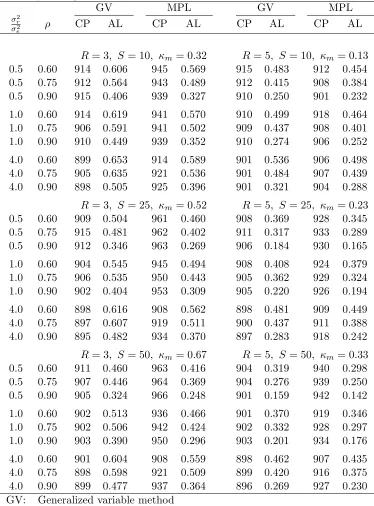
If we have no prior information of δ, then we can use the modified profile likelihood

(MPL) approach with the estimated values ofκm corresponding toδU = 16 in Table 3.1 The

resulting confidence intervals are conservative, but their average lengths are still significantly

shorter than that by the GV method, as shown in Table 4.3.

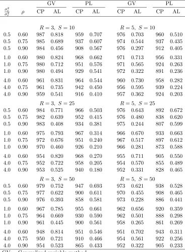
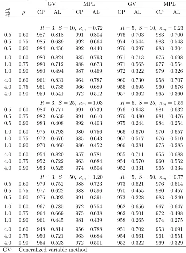
The results for one-sided lower bounds are similar. See Tables 4.4 - 4.6. Since ρ is

bounded by one from above, a one-sided lower bound and one constitute a confidence interval

for ρ. Thus, the average length of such confidence intervals, (which is equal to one minus

the average of the one-sided lower bounds), is a good measure to assess the accuracy of a

method that produces one-sided lower bounds. The average lengths (AL) in Tables 4.4 - 4.6

Table 4.2. Empirical probabilities (×1000) and average lengths of approximate 90% confi-dence intervals for ρ(based on 20,000 simulations) as well as the estimates of κ. For the PL method, κ= ˆκopt.

GV PL GV PL

σ2r

σ2

e ρ CP AL CP AL κˆopt CP AL CP AL ˆκopt

R= 3, S= 10 R = 5, S= 10

0.5 0.60 914 0.606 904 0.498 0.00 915 0.483 900 0.439 0.05

0.5 0.75 912 0.564 900 0.421 0.01 912 0.415 901 0.379 0.10

0.5 0.90 915 0.406 900 0.270 0.03 910 0.250 901 0.228 0.11

1.0 0.60 914 0.619 901 0.504 0.03 910 0.499 901 0.450 0.06

1.0 0.75 906 0.591 900 0.433 0.01 909 0.437 901 0.385 0.04

1.0 0.90 910 0.449 900 0.294 0.04 910 0.274 902 0.251 0.12

4.0 0.60 899 0.653 901 0.570 0.24 901 0.536 900 0.489 0.09

4.0 0.75 905 0.635 901 0.501 0.17 901 0.484 903 0.433 0.10

4.0 0.90 898 0.505 900 0.356 0.15 901 0.321 901 0.290 0.13

R= 3, S= 25 R = 5, S= 25

0.5 0.60 909 0.504 901 0.364 0.01 908 0.369 903 0.310 0.00

0.5 0.75 915 0.481 903 0.303 0.00 911 0.317 901 0.254 0.00

0.5 0.90 912 0.346 906 0.183 0.00 906 0.184 900 0.142 0.00

1.0 0.60 904 0.545 901 0.417 0.13 908 0.408 900 0.349 0.05

1.0 0.75 906 0.535 901 0.359 0.12 905 0.362 900 0.295 0.05

1.0 0.90 902 0.404 901 0.227 0.08 905 0.220 901 0.171 0.03

4.0 0.60 898 0.616 901 0.547 0.44 898 0.481 900 0.436 0.17

4.0 0.75 897 0.607 901 0.480 0.38 900 0.437 901 0.368 0.12

4.0 0.90 895 0.482 901 0.305 0.22 897 0.283 901 0.223 0.09

R= 3, S= 50 R = 5, S= 50

0.5 0.60 911 0.460 900 0.315 0.09 904 0.319 902 0.256 0.03

0.5 0.75 907 0.446 900 0.262 0.07 904 0.276 900 0.209 0.02

0.5 0.90 905 0.324 900 0.152 0.02 901 0.159 901 0.115 0.01

1.0 0.60 902 0.513 900 0.408 0.35 901 0.370 901 0.316 0.14

1.0 0.75 902 0.506 901 0.351 0.29 902 0.332 900 0.266 0.13

1.0 0.90 903 0.390 900 0.211 0.18 903 0.201 901 0.152 0.10

4.0 0.60 901 0.604 901 0.546 0.60 898 0.462 901 0.427 0.29

4.0 0.75 898 0.598 901 0.481 0.53 899 0.420 901 0.358 0.24

4.0 0.90 899 0.477 901 0.297 0.33 896 0.269 901 0.203 0.13

GV: Generalized variable method

PL: profile-likelihood method

CP: coverage probability

Table 4.3. Empirical probabilities (×1000) and average lengths of approximate 90% confi-dence intervals for ρ(based on 20,000 simulations). For the MPL method, κm equals to the

estimates corresponding toδU = 16 in Table 3.1.

GV MPL GV MPL

σ2

r

σ2

e ρ CP AL CP AL CP AL CP AL

R= 3, S= 10, κm= 0.32 R = 5, S= 10, κm = 0.13

0.5 0.60 914 0.606 945 0.569 915 0.483 912 0.454

0.5 0.75 912 0.564 943 0.489 912 0.415 908 0.384

0.5 0.90 915 0.406 939 0.327 910 0.250 901 0.232

1.0 0.60 914 0.619 941 0.570 910 0.499 918 0.464

1.0 0.75 906 0.591 941 0.502 909 0.437 908 0.401

1.0 0.90 910 0.449 939 0.352 910 0.274 906 0.252

4.0 0.60 899 0.653 914 0.589 901 0.536 906 0.498

4.0 0.75 905 0.635 921 0.536 901 0.484 907 0.439

4.0 0.90 898 0.505 925 0.396 901 0.321 904 0.288

R= 3, S= 25, κm= 0.52 R = 5, S= 25, κm = 0.23

0.5 0.60 909 0.504 961 0.460 908 0.369 928 0.345

0.5 0.75 915 0.481 962 0.402 911 0.317 933 0.289

0.5 0.90 912 0.346 963 0.269 906 0.184 930 0.165

1.0 0.60 904 0.545 945 0.494 908 0.408 924 0.379

1.0 0.75 906 0.535 950 0.443 905 0.362 929 0.324

1.0 0.90 902 0.404 953 0.309 905 0.220 926 0.194

4.0 0.60 898 0.616 908 0.562 898 0.481 909 0.449

4.0 0.75 897 0.607 919 0.511 900 0.437 911 0.388

4.0 0.90 895 0.482 934 0.370 897 0.283 918 0.242

R= 3, S= 50, κm= 0.67 R = 5, S= 50, κm = 0.33

0.5 0.60 911 0.460 963 0.416 904 0.319 940 0.298

0.5 0.75 907 0.446 964 0.369 904 0.276 939 0.250

0.5 0.90 905 0.324 966 0.248 901 0.159 942 0.142

1.0 0.60 902 0.513 936 0.466 901 0.370 919 0.346

1.0 0.75 902 0.506 942 0.424 902 0.332 928 0.297

1.0 0.90 903 0.390 950 0.296 903 0.201 934 0.176

4.0 0.60 901 0.604 908 0.559 898 0.462 907 0.435

4.0 0.75 898 0.598 921 0.509 899 0.420 916 0.375

4.0 0.90 899 0.477 937 0.364 896 0.269 927 0.230

GV: Generalized variable method

PL: profile-likelihood method

CP: coverage probability

Table 4.4. Empirical probabilities (×1000) and “average lengths” of approximate 95% confidence lower bounds forρ (based on 20,000 simulations). For the PL method, κ= 0.

GV PL GV PL

σ2

r

σ2

e ρ CP AL CP AL CP AL CP AL

R= 3, S= 10 R= 5, S = 10

0.5 0.60 987 0.818 959 0.707 976 0.703 960 0.510

0.5 0.75 985 0.689 937 0.607 974 0.544 937 0.435

0.5 0.90 984 0.456 908 0.567 976 0.297 912 0.405

1.0 0.60 980 0.824 968 0.662 971 0.713 956 0.331

1.0 0.75 980 0.712 951 0.576 971 0.565 924 0.263

1.0 0.90 980 0.494 929 0.541 972 0.322 891 0.236

4.0 0.60 961 0.831 964 0.544 960 0.730 958 0.282

4.0 0.75 961 0.735 942 0.450 956 0.595 939 0.224

4.0 0.90 959 0.541 916 0.410 957 0.362 924 0.203

R= 3, S= 25 R= 5, S = 25

0.5 0.60 984 0.771 966 0.503 976 0.643 892 0.672

0.5 0.75 982 0.639 952 0.415 976 0.480 838 0.620

0.5 0.90 983 0.408 934 0.381 975 0.244 807 0.599

1.0 0.60 975 0.793 967 0.314 966 0.670 933 0.663

1.0 0.75 972 0.676 951 0.240 967 0.517 897 0.612

1.0 0.90 970 0.460 926 0.210 966 0.281 873 0.588

4.0 0.60 954 0.820 968 0.270 955 0.711 905 0.550

4.0 0.75 952 0.722 958 0.205 954 0.570 855 0.489

4.0 0.90 953 0.525 940 0.180 952 0.331 828 0.465

R= 3, S= 50 R= 5, S = 50

0.5 0.60 979 0.752 947 0.693 973 0.621 938 0.528

0.5 0.75 977 0.622 900 0.611 970 0.455 908 0.465

0.5 0.90 976 0.393 858 0.581 973 0.228 886 0.441

1.0 0.60 967 0.785 955 0.661 962 0.656 920 0.359

1.0 0.75 964 0.669 930 0.590 962 0.501 888 0.298

1.0 0.90 961 0.445 900 0.561 958 0.265 861 0.269

4.0 0.60 948 0.814 951 0.546 951 0.702 943 0.311

4.0 0.75 950 0.721 910 0.466 954 0.561 922 0.256

4.0 0.90 954 0.523 865 0.433 952 0.322 905 0.233

GV: Generalized variable method

PL: profile-likelihood method

CP: coverage probability

Table 4.5. Empirical probabilities (×1000) and average lengths of approximate 95% confi-dence lower bounds forρ (based on 20,000 simulations) as well as the estimates ofκcorr. For

the PL method, κ= ˆκopt.

GV PL GV PL

σr2

σ2

e ρ CP AL CP AL ˆκopt CP AL CP AL κˆopt

R= 3, S = 10 R = 5, S= 10

0.5 0.60 987 0.818 950 0.690 -0.12 976 0.703 951 0.641 -0.20

0.5 0.75 985 0.689 950 0.519 -0.14 974 0.544 952 0.476 -0.20

0.5 0.90 984 0.456 951 0.282 -0.20 976 0.297 951 0.476 -0.20

1.0 0.60 980 0.824 950 0.703 0.05 971 0.713 950 0.651 -0.08

1.0 0.75 980 0.712 951 0.547 0.00 971 0.565 950 0.493 -0.13

1.0 0.90 980 0.494 951 0.325 -0.40 972 0.322 951 0.267 -0.14

4.0 0.60 961 0.831 951 0.758 0.51 960 0.730 951 0.692 0.19

4.0 0.75 961 0.735 951 0.638 0.43 956 0.595 950 0.547 0.15

4.0 0.90 959 0.541 951 0.437 0.36 957 0.362 950 0.324 0.03

R= 3, S = 25 R = 5, S= 25

0.5 0.60 984 0.771 950 0.621 0.10 976 0.643 951 0.580 0.02

0.5 0.75 982 0.639 950 0.459 0.07 976 0.480 950 0.412 -0.01

0.5 0.90 983 0.408 950 0.243 0.02 975 0.244 951 0.200 -0.06

1.0 0.60 975 0.793 950 0.675 0.40 966 0.670 950 0.620 0.26

1.0 0.75 972 0.676 950 0.529 0.35 967 0.517 951 0.463 0.23

1.0 0.90 970 0.460 950 0.306 0.26 966 0.281 950 0.238 0.14

4.0 0.60 954 0.820 950 0.766 0.90 955 0.711 951 0.684 0.53

4.0 0.75 952 0.722 950 0.641 0.77 954 0.570 950 0.531 0.44

4.0 0.90 953 0.525 951 0.419 0.61 952 0.331 951 0.298 0.33

R= 3, S = 50 R = 5, S= 50

0.5 0.60 979 0.752 950 0.617 0.38 973 0.621 950 0.565 0.24

0.5 0.75 977 0.622 950 0.458 0.32 970 0.455 950 0.399 0.20

0.5 0.90 976 0.393 951 0.239 0.23 973 0.228 950 0.188 0.10

1.0 0.60 967 0.785 950 0.755 1.07 962 0.656 950 0.615 0.47

1.0 0.75 964 0.669 950 0.556 0.71 962 0.501 951 0.458 0.43

1.0 0.90 961 0.445 950 0.317 0.53 958 0.265 950 0.229 0.30

4.0 0.60 948 0.814 950 0.776 1.12 951 0.702 950 0.687 0.75

4.0 0.75 950 0.721 950 0.649 0.96 954 0.561 950 0.529 0.62

4.0 0.90 954 0.523 950 0.421 0.79 952 0.322 950 0.289 0.45

GV: Generalized variable method

PL: profile-likelihood method

CP: coverage probability

Table 4.6. Empirical probabilities (×1000) and average lengths of approximate 90% confi-dence lower bounds for ρ (based on 20,000 simulations). For the MPL method, κm equals

to the values corresponding to δU = 16 in Table 3.1.

GV MPL GV MPL

σ2

r

σ2

e ρ CP AL CP AL CP AL CP AL

R= 3, S= 10, κm= 0.72 R = 5, S= 10, κm = 0.23

0.5 0.60 987 0.818 991 0.804 976 0.703 983 0.700

0.5 0.75 985 0.689 992 0.664 974 0.544 983 0.543

0.5 0.90 984 0.456 992 0.440 976 0.297 983 0.304

1.0 0.60 980 0.824 985 0.793 971 0.713 975 0.698

1.0 0.75 980 0.712 988 0.673 971 0.565 977 0.554

1.0 0.90 980 0.494 987 0.469 972 0.322 979 0.326

4.0 0.60 961 0.831 964 0.787 960 0.730 958 0.707

4.0 0.75 961 0.735 966 0.689 956 0.595 960 0.576

4.0 0.90 959 0.541 972 0.512 957 0.362 965 0.360

R= 3, S= 25, κm= 1.03 R = 5, S= 25, κm = 0.59

0.5 0.60 984 0.771 991 0.739 976 0.643 981 0.632

0.5 0.75 982 0.639 991 0.610 976 0.480 981 0.476

0.5 0.90 983 0.408 992 0.403 975 0.244 984 0.254

1.0 0.60 975 0.793 980 0.756 966 0.670 970 0.657

1.0 0.75 972 0.676 985 0.643 967 0.517 976 0.510

1.0 0.90 970 0.460 986 0.452 966 0.281 975 0.285

4.0 0.60 954 0.820 957 0.781 955 0.711 955 0.688

4.0 0.75 952 0.722 963 0.684 954 0.570 960 0.552

4.0 0.90 953 0.525 974 0.504 952 0.331 965 0.334

R= 3, S= 50, κm= 1.20 R = 5, S= 50, κm = 0.77

0.5 0.60 979 0.752 988 0.723 973 0.621 976 0.614

0.5 0.75 977 0.622 988 0.596 970 0.455 980 0.457

0.5 0.90 976 0.393 991 0.391 973 0.228 983 0.240

1.0 0.60 967 0.785 972 0.754 962 0.656 967 0.647

1.0 0.75 964 0.669 975 0.638 962 0.501 972 0.498

1.0 0.90 961 0.445 981 0.439 958 0.265 974 0.275

4.0 0.60 948 0.814 956 0.788 951 0.702 953 0.691

4.0 0.75 950 0.721 963 0.684 954 0.561 961 0.551

4.0 0.90 954 0.523 972 0.501 952 0.322 969 0.329

GV: Generalized variable method

PL: profile-likelihood method

CP: coverage probability

Chapter 5

EXAMPLES

Example 1. Fleiss et al.[5] conducted a reliability test for four raters (R = 4), each of

whom evaluated the teeth of ten patients (S = 10) independently and recorded the

num-ber of decayed, missing and filled surfaces of patients’ permanent teeth (DMFS score). We

estimate ρ to be 0.8987, with the estimate of rater-to-ratio error variability δ = 1.26 by

profile-likelihood(PL) method . By PL method, the two-sided 90% confidence interval is

(0.7120,0.9598), and the lower bound of 95% confidence is 0.7120. The modified

profile-likelihood method (MPL) gives a two-sided 90% confidence interval of (0.6808,0.9631) with

κ= 0.18 and the lower bound for 95% one-sided confidence interval of 0.6290 withκ= 0.47.

The data were also analyzed by [2] using the large sample approach and by [10] using the

generalized variable(GV) method. The estimate of ρ given by GV method is 0.9037, 90%

two-sided confidence interval is (0.6295,0.9614) and lower bound of one-sided 95%confidence

interval is 0.6201.

Example 2. Streiner et al.[9] have presented a example of rates’ effect on patients’ sadness

score where each of the three observers(R = 3) gave a ten points scale to measure a patient’s

sadness (S = 10). The estimate of ρ is 0.7304 by MPL method, and 90% two-sided

confi-dence interval is (0.3062,0.9023), with value of κ set as 0.29. MPL method also estimates

the 95% one-sided lower bound to be 0.2221 with κ = 0.74. GV method gives an estimate

ofρ of 0.7141, 90% two-sided confidence interval of (0.1481,0.8772) and lower bound of 95%

Example 3. Cuttie et al.[3] tested measurement reliability between two raters(R = 2)

for measuring hips and knees static flexion angles for both legs on nine (S = 18) healthy

children, when their bodies were oriented in order to define Outwalk anatomical coordinate

systems. For value h (hip static flexion) , MPL method yields a 90 % confidence interval for

ρ of (0.4653,0.9444) , while GV gives a 90% confidence interval of (0.1587,0.9221). Lower

bound for 95% test is 0.3839 by MPL method and 0.1474 by GV method. For value k (knee

static flexion), MPL method estimates two-sided 90% confidence interval and one-sided 95%

lower bound to be (0.2686,0.8889) and 0.2251, respectively, while GV gives the estimates of

(0.0536,0.8429) and 0.0495, respectively. The estimates of rater-to-ratio error variability are

less than 0.15 in both cases.

Example 4. Yi et al.[13] et al. used measurements of systolic blood pressure by observer

J on eighty-five patients (I = 3, S = 85) to show agreement across tools. Estimate of ρ is

0.9611 by MPL and 0.9615 by GV method. Length of 90% confidence interval is 0.0368 by

MPL and 0.0352 by GV approach. 95% confidence lower bound by GV method is 0.9352

while that given by MPL approach is 0.9039. The estimated value for δ is less than 0.2.

Example 5. In a study conducted by Vaid et al. [11], four different methods to segment

magnetic resonance images (MRI) of brain were utilized to measure the volumes of four

patients’ tumors.(I = 4, S = 4). The estimated value of δ is 2.18. ρ is estimated to be

0.7281 by MPL method. The 90% confidence interval is determined to be (0.2672,0.9359)

when κ= 0.45. Point estimate of ρ by GV method is 0.7644 and 90% two-sided confidence

interval is (0.2672,0.9539). For the lower bound of 95% one-sided confidence interval , MPL

Chapter 6

DISCUSSIONS AND FUTURE WORKS

In this paper, it is of interest to study the interrater reliability coefficient ρ from a

two-way random effects analysis of variance model in which every rater scores each subject.

The likelihood function is simplified, the profile-likelihood approach is derived, studied and

applied to obtain one-sided lower bounds and two-sided bounds forρ. The profile-likelihood

(PL) approach is more accurate than existing methods in the sense that it always produces

confidence intervals of shorter average lengths. However, the PL approach with κ = 0

understates the coverage probabilities in almost all cases. Fortunately, simulation study

shows that, we can increase the value ofκappropriately so that the PL approach is still more

precise than existing methods, but does not understate the coverage probabilities. A good

choice forκisκmdefined in (3.9), resulting in the modified profile likelihood (MPL) approach.

For the parameter settings in Section 4, the MPL approach is always more accurate than

the GV approach. Estimates of κm can can be obtained through Monte-Carlo simulation.

Table 3.1 gives the estimates of κm for several cases.

The MPL approach is in general conservative in the sense that the coverage probability

are in general higher than the expected coverage probability 1−α. In other words, the actual probability that the MPL approach produces correct results is higher than claimed. Thus,

from the point view of application, this feature of the MPL approach is not evil and should

be appreciated since it is also more precise than existing methods.

How conservative the MPL approach can be depends on the value of

whereρ0 andδ0are the true parameter values ofρandδ. A larger value ofκm−κcorr indicates

that the MPL approach is more conservative. For example, for the case R = 3, S = 50

and ρ0 = 0.90, δ0 = 0.5, the optimal value of κ is κcorr = 0.02 for producing two-sided 90%

confidence intervals (Table 4.2). If we have no knowledge aboutδ, we may setκm = 0.67 (the

number corresponding toδU = 16 in Table 3.1), and the MPL approach becomes substantially

conservative with the coverage probability 99.6% (Table 4.3). The MPL approach is not

always so conservative. For example, when R = 3, 5 and S = 10, the values of κcorr are

less variable (Table 4.2), so the value ofκm−κcorr is not expected to be high and the MPL

approach is less conservative than the GV method for certain parameter settings (Table 4.3).

Simulation study shows that, for fixed numberR of raters, the value ofκm−κcorr becomes

larger as the number S of subjects increases. When there are only a few raters but many

subjects, the MPL approach may be very conservative for certain parameter settings. On

the other hand, the value of κm −κcorr decreases as R increases (see Table 3.1) for fixed

number of subjects. In general, if the ratioR/S is not too low, the value ofκm−κcorr is near

to zero and the actual coverage probability of the MPLapproach is close to the expected one.

If a less conservative MPL approach is more desirable, the search for an estimate of

κm can be made on a narrower range of δ. For example, with the advance of technology,

measuring instruments may have excellent intrarater or test-rerest reliability, so the rater

component of variability in the ratings is large relative to the random error component, that

is, the value of δ is high. Therefore, we should search for an estimate of κm in the range of

high values of δ. As a result, the MPL approach is less conservative, but also more precise.

In conclusion, the modified profile likelihood approach proposed here is recommended

REFERENCES

[1] Bartko, J.J(1966). The intraclass correlation coefficient as a measure of

reliabili-ty,Psychological Reports,19,3-11.

[2] Cappelleri, J.C, and Ting, N.(2003). A modified large sample approach to

approxi-mate interval estimation for a particular intraclass correlation coefficient. Statistics in

Medicine,22, 1861-1877.

[3] Cutti, A.G.et al.(2010). ‘Outwalk’ : a protocal for clinical gait analysis based on inertial

and magnetic sensors. Medical & Biological Engineering & Computing, 48,17-25.

[4] Fleiss, J.L. and Shrout, P.E.(1978). Approximate interval estimation for a certain

intr-aclass correlation coefficient. Psychometrika, 43, 259-262.

[5] Fleiss J.L. (1986)The Design and Analysis of Clinical Experiment. Wiley: New York.

[6] Nelder, J.A., Mead, R.(1965). A simplex method for function minimization,Computer

Journal, 7,308-313.

[7] Rajaratnam, N.(1960). Reliability forumlas for independent decision data when

relia-bility data matched.Psychometrika,25,262-271.

[8] Satterthwaite, F.E.(1946). An approximate distribution of estimates of variance

com-ponents, Biometrics ,2, 110-114.

[9] Streiner, D.L., Norman, G.R.(1995) Health Measurement Scales: A Practical Guide to

Their Development and Use. Second edition. Oxford University Press, NY.

[10] Tian, L., and Cappelleri, J.C.(2003). A new approach for interval estimation and

hy-pothesis testing of a certain intraclass correlation coefficient: the generalized variable

[11] Vaidyanathan, M.et al. (1995). Comparison of supervised MRI segementation methods

for tumor volume determination during therapy. Magnetic Resonance Imaging, 5

,719-728.

[12] Weerahandi, S.(1993). Generalized confidence intervals.Journal of American Statistical

Association 88, 899-905.

[13] Yi, Q., Wang, P., and He,Y. (2008). Reliability analysis for continuous measurements:

Equivalence test for agreement.Statist. Med.,27 2816-2825.

[14] Zou, H., and McDermott, M.P.(1999). Higher-moments approaches to approximate

in-terval estimation for a certain intraclass correlation coefficient. Statistics in Medicine,

18, 2051-2061.

APPENDICES

Derivation of of Likelihood Function

In this section we will perform a series of algebraic operations for simplifying the expression

of the likelihood function. First we introduce several notations. For an integer n, let 1n

denote the n-dimensional one-vector whose components are one

1n=

         1 1 .. . 1          , (2)

In the n×n identity matrix, and Jn the n×n one-matrix

Jn =

        

1 1 · · · 1 1 1 · · · 1 . . . .

1 1 · · · 1

        

≡1n1Tn. (3)

For simplicity, the subscript n is suppressed in case of no confusion. Let yj be the data on

the jth subject:

yj =

and y is the RS-dimensional vector of all data y=          y1 y2 .. . yS          . (5)

It follows that the covariance matrix of y is the RS×RS matrix σ2_{V, where}

V =         

(1−ρs)IR+ρsJR ρrIR · · · ρrIR ρrIR (1−ρs)IR+ρsJR · · · ρrIR

. . . .

ρrIR ρrIR · · · (1−ρs)IR+ρsJR

         . (6)

Thus the log-likelihood function is given by

l =−1

2

RSln(2π) + ln|σ2V|+ (y−µ1)T(σ2V)−1(y−µ1)

=−1

2

RSln(2π) +RSlnσ2 + ln|V|+ (y−µ1)

T_V−1_(y−µ1) σ2

(7)

and

−2l=RSln(2π) +RSlnσ2+ ln|V|+ (y−µ1)

T_V−1_(y−µ1)

σ2 . (8)

Setting to zero the partial derivative of −2l with respect toµ

∂(−2l)

∂µ =−

2 σ2(1

T_V−1_y−µ1T_V−1_{1). (9)}

gives the maximum likelihood estimator (MLE) ˆµof µ

ˆ µ= 1

T_V−1 y 1T_V−1₁ =

1Ty

since the vector1is an eigenvalue of the matrixV−1 (andV). Similarly, equating with zero

the partial derivative of −2l with respect toσ2

∂(−2l) ∂σ2 =

RS σ2 −

(1T_V−1_y−µ1T_V−1₁₎

(σ2₎2 (11)

yields the MLE ˆσ2 _{of σ}2

ˆ

σ2 ₌ (y−µ1)

T_V−1_(y−µ1)

RS . (12)

Replace µby its maximum likelihood estimate ¯y··, we shall have

ˆ

σ2 ₌ (y−y¯··1)

T_V−1_{(y−y¯··1)}

RS . (13)

Let

∆def= (y−y¯··1)TV−1(y−y¯··1), (14)

then

ˆ σ2 ₌ ∆

RS, (15)

and

l=−1

2

RSln(2π) +RSlnσ2+ ln|V|+ ∆ σ2

, (16)

−2l=RSln(2π) +RSlnσ2+ ln|V|+ ∆

σ2. (17)

The nuisance parameter µis not involved in (14), (15), (16) and (17).

For an integer n, let h(n)₁ , h(n)₂ , . . . , h(n)n be the n×1 vectors given by

h(n)₁ =d(n)₁

               1 1 1 1 .. . 1               

, h(n)₂ =d2

               1 −1 0 0 .. . 0               

, h(n)₃ =d3

               1 1 −2 0 .. . 0               

, . . . , h(n)_n =dn

               1 1 1 .. . 1

−(n−1)

               , (18) where

d(n)₁ = √1

n, di = 1

p

(i−1)i for i= 2, . . . , n. (19)

The superscript (n) _{is suppressed if no confusion arises from this omission. Then the vectors}

{hi}ni=1 are eigenvectors of the matrix Jn. Indeed,

Jnh1 =nh1, Jnh2 = 0 for all i= 2, . . . , n. (20)

The matrix

Hn =

h

h1 h2 . . . hn

i

(21)

is the n×n orthogonal matrix due to Helmert. Now for i= 1, 2, . . . , R, let

qi1 =d (S) 1               

h(R)_i

h(R)_i

h(R)_i

h(R)_i .. .

h(R)_i

              

, qi2 =d2

              

h(R)_i

−h(R)_i 0 0 .. . 0               

, qi3 =d3

              

h(R)_i

h(R)_i

−2h(R)_i 0 .. . 0               

, . . . , qiS =dS

              

h(R)_i

h(R)_i

h(R)_i .. .

h(R)_i

−(S−1)h(R)_i

then the matrix Q given by

Q=hq11 . . . q1S; q21 . . . q2S; . . . ; qR1 . . . qRS

i

(23)

is orthogonal. Furthermore,

Vq11= [1−ρs−ρr+Rρs+Sρr]q11 (24)

Vq1j = [1−ρs−ρr+Rρs]q1j for j = 2, 3, . . . , S (25)

Vqi1 = [1−ρs−ρr+Sρr]qi1 fori= 2, 3, . . . , R (26)

Vqij = [1−ρs−ρr]qij fori= 2, 3, . . . , R and j = 2, 3, . . . , S, (27)

by (20), so qij’s are the eigenvectors of V and

λ1 def

= 1−ρs−ρr+Rρs+Sρr, (28)

λ2 def

= 1−ρs−ρr+Rρs, (29)

λ3 def

= 1−ρs−ρr+Sρr, (30)

λ4 def

= 1−ρs−ρr, (31)

are the eigenvalues of the matrix V.

Define two diagonal S×S matrices Λ1 and Λ2 by

Λ1 =

           

λ1 0 0 . . . 0

0 λ2 0 . . . 0

0 0 λ2 . . . 0

. . . .

0 0 0 . . . λ2

           

and Λ2 =

           

λ3 0 0 . . . 0

0 λ4 0 . . . 0

0 0 λ4 . . . 0

. . . .

0 0 0 . . . λ4

and denote by Λ the followingRS ×RS diagonal matrix Λ=            

Λ1 0 0 . . . 0

0 Λ2 0 . . . 0

0 0 Λ2 . . . 0

. . . .

0 0 0 . . . Λ2

            . (33)

It follows that

QTV Q=Λ and V−1 =QΛ−1QT. (34)

Since Qis orthogonal, the determinant of the matrix V is

|V|=|Λ|=|Λ1| × |Λ2|R−1 =λ1×λS2−1×λ R−1 3 ×λ

(R−1)(S−1)

4 . (35)

It follows that from (34) that

∆ = (y−y¯··1)TQΛ−1QT(y−y¯··1) = [QT(y−y¯··1)]TΛ−1[QT(y−y¯··1)]. (36)

Definez def= QT(y−y¯··1), then

∆ = z

2 (1) λ1

+

PS

j=2z2(j) λ2

+

PR

i=2z2(S(i−1)+1) λ3

+

PR

i=2

PS

j=2z2(S(i−1)+j) λ4 = a λ1 + b λ2 + c λ3 + d λ4 , (37)

where z(k) denotes the kth component of z and

a=z₍₁₎2 , b=

S

X

j=2

z_(j)2 , c=

R

X

i=2

z_(S(i2 ₋₁₎₊₁₎, d=

R X i=2 S X j=2

To simplify the expressions of a, b, c and d, let xj = yj −y¯··1R for all j = 1, 2, . . . , S, x=y−y¯·· ≡(xT₁, xT₂, . . . , xT_S)T, and

w1 =x1+x2+. . .+xS ≡d (S) 1 [h

(S) 1 ]

T_x

w2 =x1−x2 ≡d (S) 2 [h

(S) 2 ]

T_x,

w3 =x1+x2−2y3 ≡d (S) 3 [h

(S) 2 ]

T_x,

. . . .

wS =x1+. . .+xS−1−(S−1)xS ≡d (S) S [h

(S) S ]

T_x,

(39)

where hT_{x is understood as}

hTx=

S

X

j=1

h(j)xj. (40)

By (22) and (39),

w1 =

        

x1·

x2·

.. .

xR·

         , (41) and

z(S(i−1)+j) =qijTx=d (S) j h

T

i wj. (42)

It follows that

hT₁w1 =

1 R ×1

T w1 =

1

S ×x·· = 0, (43)

which implies that

By (38), (42), (43) and the fact thatHS is an orthogonal matrix,

b=

S

X

j=1

(d(S)_j hT₁wj)2 = S

X

j=1

(hT₁xj)2

=

S

X

j=1

x·j

√ R 2 =R S X j=1 ¯ x2_·j

=R

S

X

j=1

(¯y·j −y¯··)2 = SSBS.

(45)

By (38), (42), (43) and the fact thatHR is an orthogonal matrix,

c=

R

X

i=1

(d(S)₁ hT_i w1)2 = [d(S)1 ] 2

R

X

i=1

(hT_i w1)2

= 1

S ×(HRw1) T_H

Rw1 =

1 S ×w

T 1w1

= 1

S R

X

i=1

x2_i· =S R

X

i=1

¯ x2_i·

=S R

X

i=1

(¯yi·−y¯··)2 = SSBR.

(46)

By the proof of (45) and (46),

SSBS =

S

X

j=1

(d(S)_j hT₁wj)2, (47)

SSBR =

R

X

i=1

(d(S)₁ hT_iw1)2. (48)

Using the fact that HS is orthogonal again yields that

S

X

j=1

(d(S)_j hT_i wj)2 = S

X

j=1

Thus, by (38), (42), (43), (47), (48) and (49), d= R X i=2 S X j=2

(d(S)_j hT_i wj)2

= R X i=1 S X j=1

(d(S)_j hT_i wj)2− S

X

j=1

(d(S)_j hT₁wj)2− R

X

i=1

(d(S)₁ hT_i w1)2

= R X i=1 S X j=1

(hT_i xj)2−SSBS−SSBR

=

S

X

j=1

(HRxj)T(HRxj)−SSBS−SSBR

=

S

X

j=1

xT_jxj −SSBS−SSBR

= TOT−SSBS−SSBR = SSE.

(50)

Hence,

∆ = SSBS

λ2 +SSBR λ3 +SSE λ4 , (51) and ˆ σ2 ₌ ∆

RS = 1 RS SSBS λ2 + SSBR λ3 + SSE λ4 . (52)

It follows that the log-likelihood function is

l =−1

2

RSln(2π) +RSlnσ2

+ lnλ1+ (S−1) lnλ2+ (R−1) lnλ3+ (R−1)(S−1) lnλ4

which implies that SSBS, SSBR and SSE are mutually independent. Furthermore, for true

parameter values, the distributions of

SSBS λ2σ2

, SSBR

λ3σ2

and SSE

λ4σ2

(54)

are Chi-square distributions with degrees of freedom S −1, R −1 and (R −1)(S − 1), respectively. It is easy to verify that

θS =λ2σ2, θR=λ3σ2, σe2 =λ4σ2. (55)

Replacing σ2 _{in (53) by its MLE in (52) yields the following log-likelihood function of}

ρs and ρr:

l=−1

2[c0+D(λ1, λ2, λ3, λ4) +RSln ∆]

=−1

2

c0+D(λ1, λ2, λ3, λ4) +RSln(

SSBS λ2

+ SSBR

λ3

+ SSE

λ4

)

,

(56)

where

c0 = (1 + ln 2π−lnRS)RS, (57)

D(λ1, λ2, λ3, λ4) = lnλ1+ (S−1) lnλ2+ (R−1) lnλ3+ (R−1)(S−1) lnλ4. (58)

The constant c0 is free of parameters, and D = D(λ1, λ2, λ3, λ4) is the determinant of the

matrix V.

A notable fact is that, the log-likelihood function in (56) depends on only on the two