A likelihood framework for deterministic hydrological models and the importance of non stationary autocorrelation

https://doi.org/10.5194/hess-23-2147-2019 © Author(s) 2019. This work is distributed under the Creative Commons Attribution 4.0 License.

A likelihood framework for deterministic hydrological models and

the importance of non-stationary autocorrelation

Lorenz Ammann1,2, Fabrizio Fenicia1, and Peter Reichert1,2

1_{Swiss Federal Institute of Aquatic Science and Technology (Eawag), Dubendorf, Switzerland} 2_{Department of Environmental Systems Science, ETH Zurich, Zurich, Switzerland}

Correspondence:Lorenz Ammann ([email protected]) Received: 27 July 2018 – Discussion started: 13 August 2018

Revised: 25 March 2019 – Accepted: 26 March 2019 – Published: 30 April 2019

Abstract. The widespread application of deterministic hy-drological models in research and practice calls for suitable methods to describe their uncertainty. The errors of those models are often heteroscedastic, non-Gaussian and corre-lated due to the memory effect of errors in state variables. Still, residual error models are usually highly simplified, of-ten neglecting some of the mentioned characteristics. This is partly because general approaches to account for all of those characteristics are lacking, and partly because the benefits of more complex error models in terms of achieving better pre-dictions are unclear. For example, the joint inference of auto-correlation of errors and hydrological model parameters has been shown to lead to poor predictions. This study presents a framework for likelihood functions for deterministic hydro-logical models that considers correlated errors and allows for an arbitrary probability distribution of observed streamflow. The choice of this distribution reflects prior knowledge about non-normality of the errors. The framework was used to eval-uate increasingly complex error models with data of vary-ing temporal resolution (daily to hourly) in two catchments. We found that (1) the joint inference of hydrological and er-ror model parameters leads to poor predictions when con-ventional error models with stationary correlation are used, which confirms previous studies; (2) the quality of these pre-dictions worsens with higher temporal resolution of the data; (3) accounting for a non-stationary autocorrelation of the er-rors, i.e. allowing it to vary between wet and dry periods, largely alleviates the observed problems; and (4) accounting for autocorrelation leads to more realistic model output, as shown by signatures such as the flashiness index. Overall, this study contributes to a better description of residual er-rors of deterministic hydrological models.

1 Introduction

Deterministic hydrological models are widely applied in re-search and decision-making processes. The quantification of their associated uncertainties is therefore an important task with high relevance for the scientific learning process, as well as for operational decisions with respect to water man-agement. The total output uncertainty of those models is a combination of (i) propagated input uncertainty (e.g. Sun et al., 2000; Kavetski et al., 2003; Bárdossy and Das, 2008); (ii) model structural errors (e.g. Butts et al., 2004), which can be attributed to aggregation and parameterisation; and (iii) parameter uncertainty (e.g. Freer et al., 1996; Wagener et al., 2001). When performing inference, (iv) observation errors are an additional source of uncertainty, which arise for example due to errors in rating curves (e.g. Kuczera and Franks, 2002). The sources (i–iv) usually result in residual errors of predicted streamflow observations with the follow-ing characteristics:

– Non-stationarity.Model residuals can have very differ-ent characteristics in time. For example, during wet pe-riods dominated by rainfall, errors are generally less correlated than during dry periods (Yang et al., 2007). Schaefli et al. (2007) find that residuals are less cor-related during high flows than during low flows in a glacierised alpine catchment.

– Unequally spaced observations.Observations do not al-ways take place at fixed time intervals. Particularly for water quality, volume-proportional sampling strategies are generally preferable to fixed-time strategies (e.g. Schleppi et al., 2006). These strategies generate obser-vations at unequal time intervals. Another cause of un-equal observation intervals is missing data.

Various studies have investigated error models that con-sider correlation, heteroscedasticity and non-normality of errors of deterministic hydrological models. A typical ap-proach, which is also applied in this study, is to describe total output uncertainty in a lumped way (e.g. Schoups and Vrugt, 2010; McInerney et al., 2017). Another group of ap-proaches distinguishes among the different sources of total uncertainty such as input, parametric and output measure-ment uncertainty (e.g. Kavetski et al., 2006; Renard et al., 2010). The latter approach is conceptually desirable, but it can lead to identifiability problems and it is computation-ally very intensive due to the required propagation of errors through the model. For many applications we need a com-putationally cheaper approach that can be achieved with a lumped model. It is the goal of this paper to contribute to the improvement of these lumped approaches. Current ap-proaches to describe total output uncertainty in a lumped way differ in if, and how, they deal with the various characteris-tics of residual errors mentioned above. Some of the most common approaches are the following:

– Heteroscedasticity is often considered in weighted least-squares error models by parameterising the vari-ance of the normal distribution as a function of the streamflow (Thyer et al., 2009; Evin et al., 2013; Bertuzzo et al., 2013). Another common approach is to apply transformations such as Box–Cox to the ob-served and modelled streamflow time series and for-mulate a model for the residuals of the transformed time series (e.g. Bates and Campbell, 2001; Del Giu-dice et al., 2013; McInerney et al., 2017). However, this transformation affects several properties of the residuals simultaneously, including heteroscedasticity, skewness and kurtosis.

– Typically, residual errors are represented as a stationary process. The issue of stationarity has been the subject of recent debate (Milly et al., 2008; Montanari and Kout-soyiannis, 2014). Focusing on streamflow dynamics, an example of representing non-stationarity of residual er-rors is shown in the study of Yang et al. (2007), who

distinguish between wet and dry periods by applying a continuous autoregressive process with different param-eters for the wet and the dry periods to the Box–Cox transformed residuals.

– A probabilistic model to deal with unequally spaced data was proposed by Duan et al. (1988). A more nat-ural formulation is to adopt a continuous-time formula-tion of the autoregressive model, such as an Ornstein– Uhlenbeck process (OU process; e.g. Kloeden and Platen, 1995; Yang et al., 2007).

– Non-negativity of streamflow can be addressed by trun-cating the error probability density function so that it does not extend to negative streamflow. This leads to zero probability for zero streamflow, which may not al-ways be adequate. The truncation approach is seldom followed, and in most applications the truncation occurs “in prediction only” (McInerney et al., 2017).

Residual error models are usually highly simplified, in the sense that they do not account for all the above-mentioned characteristics of these errors. In particular, residual er-ror models seldom go beyond using “variance stabilisa-tion” techniques such as Box–Cox transformations. The widespread use of relatively simple error models is due to several reasons. In our opinion, the following are the most important.

trans-formation parameters or distributions of the innovations of residuals.

Second, there is limited guidance to the choice of a par-ticular error model for a given application. In the past, the choice has been generally ad hoc, with limited justification. Only recently, there has been more systematic comparison and testing which has resulted in some general recommen-dations. For example, McInerney et al. (2017) compare vari-ous residual error schemes, including standard and weighted least squares, the Box–Cox transformation (with fixed and calibrated power parameter) and the log-sinh transformation using data from 23 catchments and concluded that Box–Cox has on average the best behaviour.

Third, previous experience has shown that more realistic error models, which are more complex, do not always re-sult in better predictions. The additional parameters of some of the more complex error models were found to have un-desirable interactions with the parameters of the hydrologi-cal model, leading to unrealistic parameter values and poor predictions. For example, particularly in dry catchments, ac-counting for autocorrelation produces worse predictions than omitting it (Schoups and Vrugt, 2010; Evin et al., 2013). To circumvent such problems, Evin et al. (2014) recommend that autoregressive parameters are inferred sequentially, that is, after having estimated all other parameters of the hydro-logical and of the error model. Similarly, many uncertainty analysis techniques are applied for fixed hydrological param-eters, avoiding the re-calibration of hydrological models (e.g. Montanari and Brath, 2004). The joint inference of hydrolog-ical and error model parameters remains conceptually prefer-able, as it recognises potential interactions between parame-ters. The conditions under which this can be achieved remain poorly understood.

Fourth, the potential advantages of more complex error models are under-appreciated by the hydrological commu-nity. For relatively simple uncertainty analysis, like the plot-ting of uncertainty bands around hydrographs, the use of sim-plified error models may appear justified. However, there are several applications that go beyond this task, and for which a simplified error model may lead to poor results. For ex-ample, assuming uncorrelated errors may lead to unrealistic extrapolations (Del Giudice et al., 2013) or too-strong short-term fluctuations, which have a large effect on hydrograph signatures that are sensitive to noise, such as the flashiness index (Baker et al., 2004; Fenicia et al., 2018). The ability to correctly represent signatures is not only important for con-ceptual reasons, but also for practical purposes such as in signature-based model calibration.

The goals of this study are the following:

1. Develop a flexible framework for likelihood functions for hydrological models that accounts for the following major characteristics of their errors: non-normality (het-eroscedasticity, skewness and excess kurtosis), autocor-relation, non-stationarity regarding wet and dry

peri-ods, unequally spaced observation time points, and non-negativity of streamflow.

2. Use the flexible framework to do controlled experiments by varying some of the assumptions and by perform-ing joint inference of a hydrological model with error models of increasing complexity. Investigate the effect of the various assumptions on the quality of the predic-tive distributions. In particular, with case studies in two catchments, we investigate the following questions:

(a) Can we confirm previous findings about the prob-lems related to joint inference of hydrological and error model parameters?

(b) What are the causes of the problems encountered in joint inference of hydrological and error model parameters?

(c) Can we improve the joint inference by introducing non-stationarity by allowing the autoregressive pa-rameter to change between wet and dry periods? (d) Does the consideration of autocorrelation lead to

more realistic predictions (e.g. in terms of better representation of hydrograph signatures such as the flashiness index)?

(e) Can parameters controlling the shape of the dis-tribution of the errors be inferred jointly with the hydrological model parameters to account for non-normality?

The paper is structured as follows. The theoretical frame-work for the probabilistic model, corresponding to Goal 1, is presented in Sect. 2.1 and the performance metrics used to evaluate it are described in Sect. 2.4. Section 3 describes the case study set-up used to carry out the necessary investiga-tions for Goal 2. The case study is based on two catchments (Sect. 3.1), one hydrological bucket model (Sect. 3.2) and three different time step sizes (daily, 6-hourly and hourly). The results of those investigations are presented in Sect. 4 and discussed in Sect. 5. Section 6 lists the main conclusions and sketches potential directions for future research.

2 Methods

2.1 Probabilistic framework

Suppose we choose the distributionDQto describe the

prob-ability of observing streamflowQ, given the model output

Bates and Campbell, 2001; Del Giudice et al., 2013; McIn-erney et al., 2017) and approaches that use non-normal inno-vations of the stochastic process (Schoups and Vrugt, 2010; Scharnagl et al., 2015), both of which lead to DQ not

be-ing readily available in closed form. In particular, discussbe-ing the possible distribution of streamflow given the output of a hydrological model is easier than discussing Box–Cox trans-formation parameters or the distribution of the innovations of the model errors. Providing explicit control overDQ

there-fore facilitates the formulation of the model based on prior knowledge resulting from past experience of hydrologists in units they are familiar with. Wani et al. (2019) present an-other approach in whichDQat subsequent output time steps

is accessed through copulas.

We assume that DQ is parameterised byQdet and some error model parameters ψ, i.e. Q(t )∼DQ(Qdet(t,θ),ψ), whereθ are the parameters of the deterministic hydrologi-cal model. This implies that the observed streamflow at dif-ferent time points can be described by difdif-ferent distributions (e.g. with varying mean and standard deviation), but these distributions belong to the same parametric family. The dis-tributionDQmay extend to negative values. In this case, the

integrated probability of negative values is assigned to the probability of observing a streamflow of zero. This leads to

pDQ(Qdet,ψ) Q

=     

fDQ(Qdet,ψ) Q

ifQ >0, FDQ(Qdet,ψ) 0

ifQ=0,

0 ifQ <0,

(1)

wherefDQandFDQare the density and cumulative

distribu-tion funcdistribu-tion ofDQ, respectively, andpis a probability

den-sity forQ >0 and a discrete probability forQ=0. Note that Eq. (1) reflects our prior knowledge thatQ≥0 when dealing with non-tidal rivers. If the distribution chosen forDQis

lim-ited to positive support, either by choosing a distribution with positive support or by truncating at zero, only the first case in Eq. (1) applies and we get zero probability for Q=0. This is a common approach that is fully covered by the presented framework. However, especially in ephemeral catchments, a finite probability forQ=0 might be desirable (Smith et al., 2010). This can be achieved by choosing a distribution DQ

that extends to negative values. Equation (1) then assigns the negative tail toQ=0. If correlation is absent or neglected, Eq. (1) can be applied at each time step and the likelihood function is simply the product of those mutually independent terms.

Accounting for temporal correlation requires some addi-tional conceptualisations. Consider the transformation func-tion

ηtrans(Q, Qdet,ψ)=F_N−₍1_0,1) FDQ(Qdet,ψ)(Q)

, (2)

which transforms the streamflow, Q, via its assumed marginal distribution,DQ, which is dependent on the model

output, Qdet. If the distributional assumptions for DQ are

correct, the result of this transformation is a standard nor-mally distributed variable. Applying Eq. (2) to a time series of streamflow,Q(ti), leads to a time series of transformed

streamflows:

η(ti)=ηtrans(Q(ti), Qdet(ti),ψ), (3)

whereti are the time points of interest for inference or

pre-diction. Note that, if the distributional assumptions aboutDQ

hold at all points in time,η(ti)are a sample from a standard

normal distribution, except for the lower tail, which can be lighter due to the truncation at zero at each individual time step.

To describe autocorrelation in the deviations of Qfrom

Qdet, we assume that the corresponding time series ofηare discrete-time results of a continuous-time autoregressive pro-cess:

η(ti)|η(ti−1)∼

N η(ti−1)exp

−ti−ti−1

τ (ti)

,

s

1−exp

−2ti−ti−1

τ (ti)

!

(4)

where N is the normal distribution and the first and the sec-ond argument is the mean and the standard deviation, respec-tively. This so-called Ornstein–Uhlenbeck process (Uhlen-beck and Ornstein, 1930) has a standard normal asymptotic distribution and a characteristic correlation time,τ (ti), that

is assumed to be constant over the interval[ti−1, ti].

In summary, to transfer information between time points, we transform the distributionDQat timeti−1to a standard normal distributionηi−1according to Eq. (2), advanceηi−1 toηi according to Eq. (4), and transformηi back toDQat

timeti.

Note that, for a constant time step1t=ti−ti−1, Eq. (4) becomes

η(ti|ti−1)∼N

η(ti−1)φ,

q

1−φ2

, (5)

with

φ=exp(−1t

τ ) or τ = −

1t

ln(φ). (6)

In order to formulate the probability of the streamflowQ, we used Eqs. (1) to (4) to derive the following conditional prob-abilities forQ(ti)givenQ(ti−1)(see Appendix A for the full derivation).

IfQ(ti−1) >0:

pi Q(ti)|Q(ti−1),θ,ψ

=                   

fDQ(Qdet(ti,θ),ψ)Q(ti)

f N

η(ti−1)exp

−ti−ti−1

τ (ti )

, r

1−exp

−2ti−ti−1

τ (ti ) (η(t_i))

fN(0,1)(η(ti))

ifQ(ti) >0, F

N

η(ti−1)exp

−ti−ti−1

τ (ti )

, r

1−exp

−2ti−ti−1

τ (ti )

(η(ti))

ifQ(ti)=0.

IfQ(ti−1)=0:

pi Q(ti)|Q(ti−1),θ,ψ

=

  

f

DQ Qdet(ti,θ),ψ

Q(t_i) if Q(t_i) >0,

F

DQ Qdet(ti,θ),ψ

(0) if Q(t_i)=0.

(7) Note thatpis a probability density (denoted byf) ifQ(ti) >

0, and an integrated, discrete probability (denoted by F) if Q(ti)=0. Note also that ηin Eq. (7) is calculated with

Eq. (3) and depends onQandQdet(θ). Furthermore, Eq. (7) reduces to Eq. (1) for(ti−ti−1)/τ→ ∞, i.e. if the charac-teristic correlation time is short compared to the length of the time step.

The likelihood is then obtained by building the product of the conditional probabilities in Eq. (7) and by substituting the observations,Qobs, forQ:

fL Qobs(t0), Qobs(t1), . . . , Qobs(tn)|θ,ψ

=

pDQ(Qdet(t0,θ),ψ) Qobs(t0)

n

Y

i=1

pi Qobs(ti)|Qobs(ti−1),θ,ψ. (8)

Note that the first term on the right hand side of Eq. (8) can be calculated with Eq. (1), since it is not conditional on the previous time step.

Zeger and Brookmeyer (1986) and Hannachi (2012) for-mulated a likelihood that allows the memory of an autore-gressive processes to be kept during time periods with cen-sored data. This concept can be transferred to the case of zero streamflow. It has a conceptual advantage over Eq. (7), especially when dealing with intermittent data with frequent periods with observations of zero that can be shorter than the characteristic correlation length, like for example in the case of precipitation (Hannachi, 2012). Depending on a catch-ment’s low-pass filtering effect, streamflow is expected to have fewer but longer continuous periods of zero and non-zero data compared to precipitation. Consequently, the mem-ory of the process given by Eq. (4) is likely to vanish during

a zero streamflow period of typical length, reducing the ben-efit of keeping the correlation during those periods. There-fore, the cost of numerically solving integrals, the dimension of which is proportional to the length of the zero streamflow period (Hannachi, 2012), outweighs the conceptual benefits with respect to this application. The approach by Zeger and Brookmeyer (1986) might be highly relevant in other hydro-logical applications, however.

2.2 Error models

As a basis for subsequent applications, we setDQ to the

skewed Student’st distribution (Fig. 1), which is obtained by transforming the conventional Student’stdistribution ac-cording to Fernandez and Steel (1998). This approach of skewing has been used in a previous study on error mod-els (Schoups and Vrugt, 2010), albeit in a different setting. Thus, we introduce two error model parameters:γ, defining the degree of skewness, anddf, the degrees of freedom as a measure for the kurtosis. The skewed Student’stdistribution reduces to the normal distribution forγ=1 and df→ ∞. Two assumptions are tested to centreDQatQdet:

E[DQ] =Qdet(t ), (9a)

mode(DQ)=Qdet(t ), (9b)

i.e. we either assign the expected value or the highest proba-bility density ofDQtoQdet. A third alternative would be to set the median ofDQequal toQdet. By testing the two op-tions in Eq. (9), we include the lowest and the highest value; the third option would be a compromise between the two and was not included in the study. If not indicated otherwise, the assumption in Eq. (9a) was used. The results obtained with Eq. (9b) can be found in Appendix B.

The standard deviation ofDQis parameterised as follows:

σDQ(t )=aQ0

_Q

det(t )

Q0

c

+bQ0. (10) Note that skewing a distribution with the approach developed by Fernandez and Steel (1998) changes its standard devia-tion;σDQ(t )is the standard deviation ofDQafter skewing.

Other parameterisations ofσDQare in principle possible; see

McInerney et al. (2017) for a theoretical correspondence with transformation approaches. McInerney et al. (2017) have shown that transformation approaches with a first-order cor-respondence toc=0.8 orc=0.5 can lead to more reliable and precise predictions than those corresponding toc=1. To limit the scope of the analysis, and to maintain comparability to previous studies (Thyer et al., 2009; Schoups and Vrugt, 2010; Evin et al., 2013), we setcequal to 1. Note that the pa-rametersaandbbecome dimensionless (and therefore more universal) by including a reference streamflow,Q0, that cor-responds to the mean of the observations:Q0=Qobs. Thus,

Table 1.Overview of the error models applied in this study, their assumptions regarding correlation and the distribution of streamflow and their corresponding parameters (SKT: skewed Student’stdistribution,×: fitted).

Error model Distribution Correlation a b γ df τmin τmax

E1 Gaussian none × × 1 ∞ 0 0

E2 Gaussian constant × × 1 ∞ =τmax ×

E3∗ Gaussian non-stationary, partially fitted × × 1 ∞ 0 ×

E3a∗ Gaussian non-stationary, fitted × × 1 ∞ × ×

E4∗ SKT non-stationary, partially fitted × × × × 0 ×

E4a∗ SKT non-stationary, fitted × × × × × ×

If∗is appended to the name of the error model, a smoothed version ofPerr(t )(moving average of window size 5 h) was used in Eq. (11).

Figure 1. Example of skewed Student’s t distributions with E[DQ] =Qdet(t )=2.5 mm h−1and standard deviationσDQ(t )= 0.6 mm h−1for different values of skewness,γ, and degrees of free-dom,df.

Table 1 lists the error models applied in this study, together with their underlying assumptions. E1 is included as a refer-ence case; it is based on the assumption of uncorrelated het-eroscedastic errors with a normal distribution. These assump-tions, with the exception of heteroscedasticity and the treat-ment ofQobs=0, are identical to those made when maximis-ing the Nash–Sutcliffe efficiency for example, or, equiva-lently, minimising the squared residuals. Error model E2 rep-resents a conventional approach to considering autocorrela-tion. In the case of equally spaced time steps, it is similar to the error model applied by Evin et al. (2013) for example, who assume that the rescaled errors follow an AR(1) process with a standard normal marginal distribution. One difference between the two approaches is, again, the treatment of cases whereQobs=0. In error model E3, we additionally account

for the fact thatτ might be time-dependent. The following formula forτ is used in those cases:

τ (t )=

(

τmin if Perr(t ) >0,

τmax otherwise,

(11)

wherePerr is the precipitation used as an input for the er-ror model. In E3,τmin is fixed at 0, while in E3a, it is fit-ted.Perr was either equal to the recorded precipitation, P, or, in the case of hourly resolution in the Maimai catchment, smoothed with a moving average of window size 5 h. This was done to prevent frequent jumps betweenτminandτmax during precipitation events, and to be more robust with re-spect to potential time lags between observed precipitation and streamflow. Note that, if such time lags were excessively large, they would have to be considered in Eq. (11). Since in the Murg catchment smoothing did not change the results substantially,Perr=P applies there. Thus, error model E3a (or E3) can be seen as a mixture of E1 and E2, in the sense thatτ alternates between periods of high and low (or no) cor-relation. Finally, E4 relaxes the assumption of normality for

DQ; we use a skewed Student’stdistribution, inferring the

degrees of freedom and the skewness. Again, E4a denotes the version whereτminis inferred.

2.3 Inference and prediction

Consider that for any practical case of inference or predic-tion, we will have a finite series of time points of interest

(t0, t1, . . ., tn) and a corresponding time series of

stream-flowQ=(Q(t0), Q(t1), . . . , Q(tn))or, in analogy,Qdetand Q_obs. When performing inference, the parameters of the hy-drological model,θ, are estimated jointly with the parameters of the error model,ψ, by evaluating the likelihood function (Eq. 8) according to the following procedure:

1. Given a suggested parameter vector θ, evaluate the deterministic hydrological model, Q_det, for all time points.

As the likelihood (Eq. 8) is available in closed form for a given output of the hydrological model, like in many com-mon likelihood functions in hydrology, we do Bayesian in-ference based on standard MCMC sampling of the posterior. The affine-invariant ensemble sampler by Foreman-Mackey et al. (2013) is used for this purpose. It uses the so-called “stretch move” to propose a new value for a point in param-eter space based on other members of the ensemble. The en-semble size consists of 100 walkers in this study and conver-gence is assessed visually. A full posterior sample consists of 10 000 model evaluations after successful convergence.

For prediction, stochastic realisations of model output are obtained by inverting Eq. (2):

Qtrans(η, Qdet,ψ)=F_D−_Q1_(Qdet,ψ) FN(0,1)(η), (12)

and applying the following procedure to produce a single stochastic streamflow realisationQ_j:

1. Randomly draw a parameter vector (θ,ψ)j from the

posterior sample.

2. Usingθj, evaluate the deterministic hydrological model

to obtainQ_{det, j}for all time points.

3. Usingτ_j∈ψ_j and Eq. (4), produce a stochastic real-isation of an OU process, η_j, with a standard normal marginal distribution.

4. Use ψ_j and Q_{det, j}, determined in steps 1 and 2, to transformη_j into a stochastic realisation of streamflow, Q_j, with Eq. (12).

Note that a simulation with the hydrological model requires some additional input like precipitation and potential evapo-transpiration data (Sect. 3.1), which is assumed to be known also for the prediction period. In a synthetic case study, we could successfully verify the consistency of the implemented likelihood and sampling functions (see the Supplement). 2.4 Evaluation criteria

How can the performance of empirical error models, such as those presented in this study, be quantified? We argue that the performance of an error model in joint inference with a hydrological model should be judged according to the following criteria: (a) good reproduction of observed dy-namic fluctuations by individual model realisations, (b) good overall predictive marginal distribution of streamflow, and (c) small absolute deviance between model output and ob-servations. The flashiness index (Sect. 2.4.1) is an indicator for (a). The reliability and the relative spread of the pre-dictive distribution (Sect. 2.4.2 and 2.4.3, respectively) are used as an indicator for (b). The Nash–Sutcliffe efficiency (Sect. 2.4.4) and the relative error in cumulative streamflow (Sect. 2.4.5) cover (c). In addition to those performance met-rics, we calculated the Kullback–Leibler divergence

(Kull-back and Leibler, 1951) of the marginal posterior parame-ter distributions from the prior according to the method pro-posed by Boltz et al. (2007).

2.4.1 Flashiness index

The function to calculate the flashiness index (Baker et al., 2004) is given by the following:

I (Q)=

Pn

i=1|Q(ti)−Q(ti−1)|

Pn i=1Q(ti)

, (13)

where Q=(Q(t0), Q(t1), . . . , Q(tn)). Let bx denote the

quantityx that is related to the hydrological parameter val-ues at the maximum posterior density. The flashiness index is calculated for the observations,IF,obs=I (Qobs); the output of the deterministic hydrological model, bIF,det=I (Qb_det);

and the individual stochastic realisations of the predictive streamflow sample,IF=median(I (Qj)). IF is sensitive to the amount of autocorrelation in a streamflow time series, as well as the height of the peaks ofQ_det(sinceQ_j depends on Q_det).

2.4.2 Reliability

Reliability is defined similarly to McInerney et al. (2017), as follows:

4reli=1− 2

n+1

n

X

i=0

|FQ(ti)(Qobs(ti))

−Fζ(FQ(ti)(Qobs(ti)))|, (14)

whereζ= {FQ(ti)(Qobs(ti))|i∈N,0≤i≤n},Fζ is the

em-pirical cumulative distribution function ofζandFQ(ti)is the

empirical cumulative distribution function of the predicted streamflow at time ti. 4reli can take values in the interval [0,1], where larger values of4reli correspond to better re-liability and unity means perfect rere-liability. It measures the degree to which the observations are consistent with being a sample of the predictive distribution. Since comparison hap-pens in the uniform space, the influence of heavy outliers on

4reliis limited. Note that we use the complement of the reli-ability measure proposed by McInerney et al. (2017), in or-der to allow for a more intuitive interpretation (larger values mean larger reliability).

2.4.3 Relative spread

The relative spread is an indicator for the width of the pre-dictive distributions over all time points, and was proposed by McInerney et al. (2017) as follows:

spread=

Pn

i=0σQ(ti)

Pn

i=0Qobs(ti)

, (15)

whereσQ(ti)is the standard deviation of the predictive

stochastic predictions at that point in time.spread∈R+, and

small values ofspreadindicate precise predictions or small predictive uncertainty. The smaller the predictive uncertainty, the better the quality of the underlying model, given that the predictions are not overconfident. While McInerney et al. (2017) use the name “precision” forspread, we believe that “relative spread” is a more appropriate term considering its actual meaning.

2.4.4 Nash–Sutcliffe efficiency

The Nash–Sutcliffe efficiency (Nash and Sutcliffe, 1970),

EN,f(f for function), is defined as follows:

EN,f(Q,Qobs)=1−

Pn

i=0(Q(ti)−Qobs(ti))2

Pn

i=0(Qobs(ti)−Qobs)2

, (16)

where Q=(Q(t0), Q(t1), . . . , Q(tn)). It is used in this

study to assess the output of the hydrological model at the maximum posterior parameter density, EbN,det=

EN,f(Qb_det,Q_obs), as well as the stochastic simulations,

EN=median(EN,f(Qj,Qobs)). It is used as a rough mea-sure of how well two hydrographs correspond to each other, primarily with the goal of identifying very poorly fitting hy-drographs. It is known to be sensitive to errors in high flows (Legates and McCabe, 1999), which can be of particular practical interest. Therefore it complements the other mea-sures, which are less informative with respect to errors in high flows.

2.4.5 Relative error in total cumulative streamflow As a measure of systematic over- or under-prediction of streamflow, we calculate the relative error in total cumula-tive streamflow:

1(Q,Q_obs)=

Pn

i=0Qobs(ti)−Q(ti)

Pn

i=0Qobs(ti)

. (17)

It is calculated with respect to the model output based on the parameter values at the maximum posterior density;

b

1Q,det=1(Qb_det,Q_obs), as well as for the ensemble of

indi-vidual stochastic simulations:1Q=median(1(Qj,Qobs)). Note that, contrary to McInerney et al. (2017),1Qis the

me-dian error of all the individual hydrograph realisations, not the error of the average hydrograph.

3 Case study set-up 3.1 Catchments and data

The probabilistic framework developed in Sect. 2.1 was tested in two case study sites, the Murg and the Maimai catchments, which are described in this section. The Murg river flows through a hilly headwater catchment in a temper-ate climtemper-ate with a size of 80 km2 in northeastern Switzer-land. Some key hydrological summary statistics are listed

in Table 2. Land use is predominantly agricultural (50 %), with forested headwaters (30 %) and a considerable propor-tion of urban areas (10 %). The mean elevapropor-tion is 652 m a.s.l., spanning from 466 to 1035 m a.s.l. Streamflow peaks can be quite sharp, especially for small events, in which base-flow conditions are reached again within just a few hours. This is potentially due to impervious areas being drained directly into the river. The data consist of hourly averages of streamflow, precipitation and potential evapotranspiration from January 1995 to December 2002. Calibration was per-formed in the first 5 years (January 1995–December 1999) and validation in the consecutive 3 years (January 2000– December 2002). Streamflow data are courtesy of the Swiss Federal Office for the Environment (FOEN). Precipitation and potential evapotranspiration are based on meteorological data (MeteoSwiss, 2018) and were processed by the Swiss Federal Institute for Forest, Snow and Landscape Research (WSL), with the preprocessing tools of PREVAH (Viviroli et al., 2009).

The Maimai experimental catchments are a set of small headwater catchments with a long history of hydrological re-search. They are located on a deeply incised hillslope on the South Island of New Zealand. The area is forested and the cli-mate is considerably more humid than in the Murg catchment (Table 2). The site was chosen for this study due to its homo-geneous characteristics and relatively simple hydrological re-sponse, which make it very suited for model evaluation and testing (e.g. Seibert and McDonnell, 2002). We use hourly data recorded in 1985–1987 in the M8 experimental catch-ment, the most intensely studied of the Maimai catchments. It has an area of ca. 7 ha with steep (34◦) slopes. The reader is referred to Brammer and McDonnell (1996) for a more detailed description of the characteristics of the M8 and the other experimental catchments. This study does not attempt to make a significant contribution to the understanding of the hillslope processes in the Maimai catchment (see McGlynn et al., 2002, for an extensive overview). Calibration was per-formed based on data from January 1985–December 1986, and validation during January–December 1987. The data were kindly provided by Jeffrey McDonnell.

Table 2.Properties of the two case study catchments. P is the precipitation andRC the runoff coefficient (calculated from cumulative streamflow and precipitation). Qobs,max,Qobs,min andQobs are the minimum, the maximum and the average streamflow, respectively.

IF,obsis the flashiness index.

Catchment Area P RC Qobs,max Qobs,min Qobs IF,obs

(km2) (mm a−1) (–) (mm h−1) (mm h−1) (mm h−1) (–)

Murg 80 1369 0.57 2.7 1×10−2 0.089 0.053

Maimai 0.07 2349 0.62 8.5 1×10−4 0.17 0.13

Figure 2.Structure of the deterministic hydrological model used in this study.Puis the precipitation andEuthe evapotranspiration.Su

represents the active water content of the unsaturated zone, whileSf

is a non-linear reservoir representing the fast flow component.

3.2 Deterministic hydrological model

The hydrological model used throughout this study is a sim-ple, lumped bucket model with two reservoirs (Fig. 2), which are meant to represent the unsaturated soil zone and the sub-surface flow being fed by it. A slower flow component is included though a linear outflow from the unsaturated zone reservoir directly. Due to its simplicity, and due to the fact that it is not clear whether the chosen model structure is suited for the studied catchment a priori, we expect sys-temic difficulties in reproducing the observed streamflow dy-namics. This is a very common situation in hydrological modelling and it will lead to correlated and potentially het-eroscedastic and non-normal errors. This allows us, in princi-ple, to test the error models (Sect. 2.2) under realistic condi-tions. The streamflow simulated by this deterministic model is denoted asQdet(t,θ)=Qs(t,θ)+Qf(t,θ), whereQs is the slow response of the model,Qfis the fast response and θ=(Ce, Smax, ku, kf)are the calibrated hydrological param-eters. The fluxes (Eu,Pu,Qu,Qs,Qf) and states (Su,Sf) of the model are given by the following:

dSu

dt =Pu−Eu−Qu−Qs, Eu=CeEp

Su

Smax(1+m) Su Smax +m

,

Qu=Pu

_S

u

Smax

β

,

Qs=kuSu, (18)

dSf

dt =Qu−Qf,

Qf=kfSfα, (19)

whereEpis the potential evapotranspiration. WhileCe,Smax,

ku and kf were inferred, m, β and α were kept fixed at 0.01, 3 and 2, respectively.mcan be seen as a smoothing parameter and m=0.01 translates to Eu≈CeEp as long asSu/Smax0.01.β=3 andα=2 were found to lead to reasonable results in both investigated catchments and were fixed due to potential interactions withSmaxandkf. The hy-drological model was implemented in SUPERFLEX (Fenicia et al., 2011; Kavetski and Fenicia, 2011), a flexible frame-work for conceptual hydrological models which uses effi-cient numerical integration schemes.

3.3 Priors

The prior distribution of the parameters was assumed to be composed of independent normal or log-normal distributions with relatively large standard deviations (see Table 3). A uni-modal distribution is the more accurate representation of our prior belief than, for example, a uniform distribution over a predefined range, since we do assume that values in the mid-dle of the suspected range are more probable than at its edge. Note that this is primarily a conceptual difference, as large standard deviations were chosen to minimise the influence of the priors on the results.

4 Results

After providing some general results, this section contains a more detailed summary of the results for each of the tested er-ror models. The complete analysis included additional erer-ror models and performance metrics, which are included in Ap-pendix B. The supplementary material contains further infor-mation on the resulting posterior density estimates of the pa-rameters and Kullback–Leibler divergences of the marginal posterior and prior parameter density estimates.

Table 3.Prior distributions of the hydrological and error model parameters applied in all the cases where the respective parameter was used. N = Gaussian normal; LN = log-normal. Where lower and upper boundaries are listed, the distribution is truncated at those values.

Parameter Distribution Unit µ σ Lower boundary Upper boundary

Ce N – 1 0.2 0.2 3

Smax LN mm 148 1086 2.7 1086

ku LN h−1 1.8×10−2 0.13 2.3×10−6 5×10−2

kf LN h−1 0.37 2.7 2.3×10−6 0.37

a LN – 0.2 0.2 – –

b LN – 0.1 0.1 1×10−2 0.5 τmax LN h 148 1086 0 2000

γ LN – 1 0.2 0.1 5

df LN – 14 17 3 –

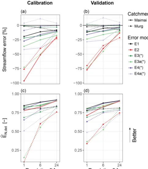
error in cumulative streamflow, 1Q, and about the Nash–

Sutcliffe efficiency, EbN,det. The temporal resolution of the data has a pronounced effect on all the analysed performance metrics. The spread over all the combinations of error mod-els and catchments is larger for higher temporal resolutions (Figs. 3 and 4). Furthermore, the average of each metric in-dicates decreasing performance for increasing temporal res-olution. This loss in performance is more pronounced in the Murg catchment and for error models E2 and E3a than in the Maimai catchment and for other error models. The difference between the two catchments is most clearly visible inEbN,det (Fig. 4): for 6-hourly and daily resolution of the data, the worst-performing error model in the Maimai catchment has a betterEbN,detthan the best-performing error model in the Murg catchment.

4.1 Individual error models

4.1.1 Model E1

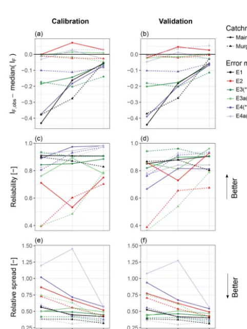
E1 tends to strongly overestimate the true flashiness in the case of high temporal resolutions in both catchments (Fig. 3a, b; the difference between the observed and the median of the predicted flashiness index is around−0.4 for both catch-ments). In terms of reliability, E1 is never the single best of the error models but is always among the best, and it is ro-bust in light of varying temporal resolution (4reliis larger or equal to 0.8 in all the cases; Fig. 3c, d). E1 is also among the error models that provide the least uncertain predictions (average relative spread of 0.41, Fig. 3e, f) and have the smallest1Q(usually between 0 % and−10 %) and the

high-est EbN,det overall (Fig. 4). Except for the flashiness index, its performance stays stable for high-frequency data in both catchments. However, the high flashiness index of this model demonstrates the strong violation in the description of the output behaviour despite its good performance regarding the other performance metrics.

Figure 3.Performance of the error models with respect to the flashi-ness index, reliability and relative spread for both catchments and all temporal resolutions.Perrwas smoothed (∗) exclusively for hourly

data in the Maimai catchment.

4.1.2 Model E2

Figure 4.Performance of the error models in terms of the relative cumulative error in streamflow, 1_Q, and the Nash–Sutcliffe effi-ciency, Eb_N,det, for both catchments and all temporal resolutions. Perrwas smoothed (∗) exclusively for hourly data in the Maimai

catchment.

output is due to the hydrological model response and only a small part is due to the stochastic variability added through the error model. Regarding all the other performance met-rics, however, E2 is often among the worst-performing error models. For example, in more than half of all the investi-gated combinations of catchments and temporal resolutions, E2 is the error model with the worst reliability (Fig. 3c, d). E2 has an average relative spread of 0.61 over all the cases, while that of E1 is 0.41. It tends to produce large errors in cumulative streamflow, especially in the case of hourly res-olution (1Q<−75 %, Fig. 4a, b). The degradation of the

streamflow error and EbN,det with increasing measurement frequency is very pronounced for E2 compared to the other error models (Fig. 4a–d).

4.1.3 Model E3

E3 generally overestimates the true flashiness; i.e.IFis often larger thanIF,obs. The difference is around 0.2 for hourly and 6-hourly resolution and a bit less for daily resolution (Fig. 3a, b). The overestimation of the flashiness by E3 is less severe than with E1. E3 results in stable reliability metrics for all temporal resolutions in both catchments:4reli is larger than 0.8 in every case and larger than 0.9 in more than half of the cases (Fig. 3c, d). In the validation period in the Murg

catchment, it is the most reliable error model of all (Fig. 3d). The relative spread of E3 is in the range of [0.34, 0.5] in all instances with an average value of 0.43, and it is unaf-fected by the temporal resolution (Fig. 3e, f). The absolute value of1Qis never larger than 25 % and usually smaller

than 10 % (Fig. 4a, b). In terms ofEbN,det, E3 reaches values larger than 0.75 in all cases except for hourly resolution in the Murg catchment, where it is 0.69. All the metrics show stable performance of E3 under increasing measurement fre-quency (Figs. 3 and 4).

4.1.4 Model E3a

When inferringτminwith error model E3a, we get close cor-respondence ofIFandIF,obsin all cases (Fig. 3a, b; the de-viation is never larger than 0.05). In the Maimai catchment, the reliability measure shows stable performance, with val-ues between 0.81 and 0.96 in the validation period (Fig. 3c, d), showing no clear signs of worse performance for high-frequency data. The inferred values ofτminwere of the order of 1 d and therefore clearly smaller thanτmax(Fig. 7). Fur-thermore,τminwas consistent among the different temporal resolutions.

In the Murg catchment, on the other hand, we see a de-generating performance of E3a with increasing measurement frequency, with values of4reli<0.5 for 6-hourly and hourly data (Fig. 3c, d), indicating poor performance. All the other metrics show a similar pattern. The inferredτminwere be-tween 50 and 100 h, where values on the upper end of that range coincided with bad reliability (Fig. 7).

4.1.5 Model E4

The stochastic model realisations with E4 tend to overesti-mate the true flashiness index; the difference betweenIF,obs andIF is usually between −0.2 and −0.1 (Fig. 3a, b). IF is often much larger thanbIF,detin the Murg catchment (Ta-ble B1), indicating that a relatively large part of the flashiness is accounted for by the error model and less by the hydrolog-ical model in that case. This manifests in smaller values of

b

EN,detwith E4 compared to E1 (e.g. 0.65 for E4 with hourly resolution compared to 0.79 with E1, Fig. 4c). In the Maimai catchment, the hydrological model captures a larger part of the variability than in the Murg catchment, and the difference betweenIFandbIF,detis smaller (Table B2). Concerning the reliability,4reliis generally larger than 0.8, indicating well-conditioned predictive distributions, except in the validation period for hourly resolution (Fig. 3c, d). In the Maimai catch-ment, reliability is better in the calibration period than in the validation period, which is a sign of over-fitting. Especially for daily resolution, E4 provides very good reliability in the calibration period in both catchments (4reli>0.97, Fig. 3c). The average relative spread of E4 is 0.60.1Q is not more

20 % (Fig. 4a, b). A slight degradation of1Qwith increasing

frequency of the data can be observed. 4.1.6 Model E4a

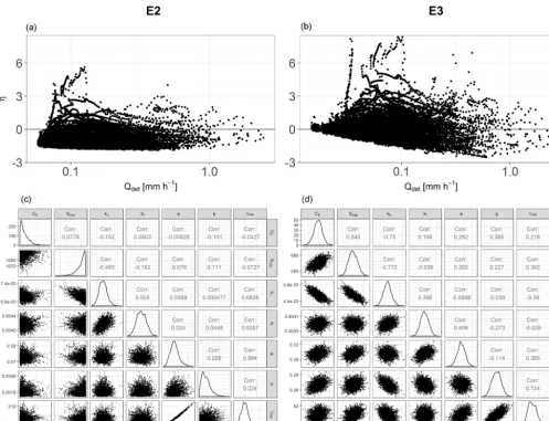
E4a results inIFthat are very close to the observed flashiness in all cases: the difference is never more extreme than 0.05 (Fig. 3a, b). bIF,det is often smaller than IF,obs in the Murg catchment, which, similar to in E4, is an indication that most of the variability is explained by the error model and not the hydrological model.4reliis always larger than 0.8 (Fig. 3c, d) except for the validation period with hourly resolution in both catchments (Fig. 3d). Similar to E4, we can see a tendency for over-fitting with E4a in the Maimai catchment: in the cal-ibration period, reliability values of 0.98, 0.95 and 0.92 are reached, while the validation results in values of 0.84, 0.84 and 0.77 for daily, 6-hourly and hourly resolutions, respec-tively (Table B2). A look at the relative spread (Fig. 3e, f) shows that E4a leads to unrealistically large prediction un-certainty in the Maimai catchment for 6-hourly and hourly resolution but that it is among the most precise error models in the Murg catchment. Similarly, E4a produces relatively large errors in cumulative streamflow in the Maimai catch-ment, but very small ones in the Murg catchment (Fig. 4a, b). Opposed to that,EbN,detis better than 0.75 in all cases in the Maimai catchment, while it reaches values as low as 0.5 for hourly resolution in the Murg catchment (Fig. 4c, d). 4.2 Relaxing the constant-correlation assumption Error model E3, which accounts for reduced correlation of errors during the precipitation events, leads to an overall improvement in the investigated performance metrics (ex-cept IF) compared to E2, which assumes constant correla-tion (Figs. 3 and 4). For example, the reliability for hourly resolution in the Murg catchment is 0.94 and 0.39 for E3 and E2, respectively (Fig. 3c, d). In contrast to E2, the per-formance of E3 does not show systematically worse perfor-mance for high-frequency data. In fact, E3 and E1 show a similar stability in performance, but E3 provides more real-istic estimates of the correlation during recessions and base-flow, leading to a better estimate ofIF (Fig. 3a, b). Figure 6 shows typical results of E2 and E3 with respect to streamflow bias, visible as a bias inη(Fig. 6a, b), and posterior corre-lation between heteroscedasticity and correcorre-lation parameters

a andτmax(Fig. 6c, d). Note also the smaller standard devi-ation (parametera) resulting from E3 (Fig. 6d). Additional results about the standardised innovations ofηare available in the Supplement.

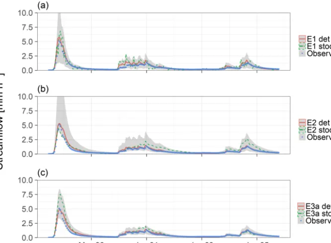
Figure 5 compares the predicted hydrographs of E1, E2 and E3a in the Maimai catchment using hourly data. In this case, allowing for different characteristic correlation times during precipitation events and dry periods (E3a, Fig. 5c) leads to better-behaved error bands compared to the con-stant correlation assumption (Fig. 5b) and to more realistic

stochastic output of the model than with the zero-correlation assumption (Fig. 5c). Note that E3a results in better estimates ofIFthan E3, since it considers correlation during precipita-tion events (τmin>0).

In the Murg Catchment, inferringτmin resulted in a de-generative performance for high-frequency data, which were also linked to higher values ofτmin(Fig. 7). The posterior es-timates ofτmaxdepend on the resolution in both catchments. While largeτmin coincides with the worst reliability, large

τmaxwas also obtained together with good reliability (Fig. 7). The effect ofτminon the relative cumulative streamflow error is shown in Fig. 8 for 6-hourly data in the Murg catchment. The streamflow error starts to increase forτmin>10 h and at the same timeEbN,detdecreases (not shown), approaching that of E2.

4.3 Relaxing the assumption of normality

Relaxing the assumption of normality by inferring γ and

df (E4 and E4a) had a mixed effect on the numeric perfor-mance indices analysed in this study. Whenτmin=0, includ-ing skewness and kurtosis (E4) often led to a better reliability in the calibration period (Fig. 3c), but a worse reliability in the validation period (Fig. 3d) compared to the assumption of a normal distribution with E3. Predictions with E4 gen-erally had a smaller spread than those with E3; e.g.spread was around 0.5 with E3 and 1.0 with E4 for hourly resolu-tion in the Maimai catchment (Fig. 3e, f). Whenτmin was inferred additionally, the non-normal case (E4a) showed bet-ter performance metrics than the normal case (E3a) in the Murg catchment, but worse ones in the Maimai catchment. E4 and E4a in the Maimai catchment were the only cases that showed a pronounced difference between calibration and validation, which is a sign of overfitting. A visual inspection of the QQ plots ofηrevealed that E4 and E4a successfully reduced some very heavy outliers that strongly violated the assumption of normality. In both catchments, the inferredγ

were in the range of[1.5,2.8]for E4 and E4a. The values at the upper end of this spectrum were reached for hourly resolutions, and they were associated with underestimation of the peak flows by the deterministic hydrological model, reflected in reduced EbN,det. For example, E4a resulted in γ≈2.5,EbN,det=0.5 and an underestimation of peak flows by the hydrological model for hourly data in the Murg catch-ment. Inferreddf were always at or close to the lower limit of 3, which is indicative of heavy outliers.

Figure 5.Streamflow predictions with hourly resolution in the Maimai catchment in a part of the validation period (1993) obtained with error models E1 (a), E2 (b) and E3a (c). Deterministic predictions with the parameter values at the maximum posterior density are shown together with the 90 %-confidence bands and one single stochastic streamflow realisation for each of the error models.

5 Discussion

5.1 Presence and absence of autocorrelation

Assumptions about the presence (E2) and absence (E1) of autocorrelation inηwere shown to have profound effects on the quality of the prediction in the cases investigated in this study. Neglecting autocorrelation leads to close correspon-dence betweenQbdetandQobsin terms of the Nash–Sutcliffe efficiency and to relatively well-fulfilled assumptions about the distribution ofηin the uniform space (i.e. small values of

4reli). However, major assumptions of the underlying statis-tical model are clearly violated. Most striking is the violation of the zero correlation assumption (Fig. 9b), which translates into unrealistic fluctuations of the stochastic streamflow pre-dictions (Fig. 5a). Note that E1 also comes with disadvan-tages related to operational forecasts, where one can make more accurate predictions for streamflow in the near future given an error in previous streamflows when accounting for correlated errors (Del Giudice et al., 2013). This effect was not analysed in this study.

Accounting for the fact thatηis obviously autocorrelated, and therefore describing it by a Gaussian process with con-stant autocorrelation (E2), comes with additional difficulties. These include a strong interaction of the hydrological water balance parameter, CE, with autocorrelation, τmax. In addi-tion, we observed a strong posterior correlation between the parameter for autocorrelation,τmax, and heteroscedasticity,a (Fig. 6c). This correlation in the posterior parameter

distri-bution coincided with systematic overprediction of stream-flow. E2 also showed smallerENandEbN,det, and worse1Q

compared to E1 (Fig. 4). Evin et al. (2013), who tested an error model similar to E2 on daily data, obtained very simi-lar results in terms of interactions of water balance parame-ters with correlation and heteroscedasticity parameparame-ters. The reasons for those problems are still poorly understood. Fail-ing to reproduce the problems under synthetic conditions, Evin et al. (2014) suggest that the “nonrobustness of the joint approach” might be caused by “structural errors in the hy-drological and/or error models”. Based on case studies with daily data, they find that (i) the catchments where these prob-lems are absent are all wet catchments with relatively high runoff coefficients and low ephemerality. To this, we can add that (ii) the performance of the corresponding error model in our study (E2) strongly degrades for higher data frequency within two relatively wet catchments.

5.2 Non-stationarity of autocorrelation

Figure 6.Transformed residuals,η, as a function of modelled streamflow(a, b)and correlation structure of the posterior parameter sample

(c, d)resulting with error models E2(a, c)and E3(b, d)for data with hourly resolution in the Murg catchment.

non-stationarity of the autocorrelation is a major deficit of conventional error models, which leads to the previously encountered problems in the joint inference of autoregressive and hydrological model parameters mentioned in Sect. 5.1. What is the physical explanation for non-stationary auto-correlation of the errorsη? The autocorrelation of errors in streamflow is primarily caused by the memory effect of er-rors in storage (Kavetski et al., 2003). Since this memory effect of a catchment during precipitation events can be ex-pected to be different from that during dry weather, the cor-relation of the errors in streamflow can be expected to be dif-ferent as well. The degree of change of the correlation may depend on multiple factors, like the hydrological model used, the precipitation intensity or volume, the extent to which the precipitation signal is filtered by the catchment, time lags be-tween precipitation and runoff, and potentially other factors. Most probably, the mentioned factors will lead to smaller

correlation during wet periods and larger ones during dry pe-riods.

A very simple way of considering this reduced correla-tion (E3) provides strongly improved results compared to the assumption of stationary correlation (Sect. 4.2). This indi-cates that neglect of the non-stationarity of the autoregres-sive parameter is a substantial shortcoming of conventional error models, which causes, at least partly, the well-known problems related to joint inference. Note that non-stationary correlation can also be implemented in other existing likeli-hood functions and does in principle not require the use of the proposed theoretical framework described in Sect. 2.1.

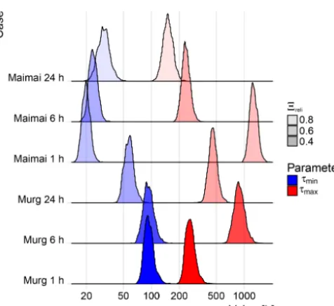
in-Figure 7.Marginal posterior densities ofτminandτmax, and

corre-sponding reliability measures4reliin the validation period resulting

from error model E3a in all combinations of catchments and tem-poral resolutions.

Figure 8.Relationship between the fixed correlation time during precipitation events,τmin, and the total streamflow error,1Q, for 6-hourly data resolution in the Murg catchment. Each point corre-sponds to a full inference and prediction procedure. The error bars span two standard deviations of 500 stochastic predictions. E3 cor-responds toτmin=0 and E2 toτmin=τmax≈170 h.

ference behaviour. To test this, we shiftedPerr(Eq. 11) sub-stantially in time, so that it would not correspond to the ob-served precipitationPanymore, while still keeping the major properties (duration and intermittency) of the time intervals during whichτ is reduced. Then, inference was performed with E3 again. The low Nash–Sutcliffe efficiency and the high streamflow error of the stochastic predictions in that case (E3† in Table B2) shows that it is indeed important

to reduce τ during the precipitation events and not during arbitrary periods with the same intermittency and duration as the precipitation events. With the shiftedPerr, the result-ingτmax(≈145 h) was much smaller than the originalτmax (≈1400 h), confirming the hypothesis of reduced correlation time of errors in streamflow during precipitation events.

One could also argue that the improved performance of E3 compared to E2 is primarily due to assuming reduced au-tocorrelation during periods with strong outliers (i.e. storm events) and that those outliers (visible in Fig. 6) should be accounted for by appropriate values of γ and df, instead of reducing their influence by neglecting correlation in the periods they appear. Or, similarly said, if the autoregres-sive process with constant correlation is applied to appropri-ately standardised residuals, which are marginally normally distributed, it should not cause any problems. To explore this possibility, we performed some experimental analysis for hourly resolution in the Murg catchment: we modified E1 by fixingγ=1.5 anddf=5 (E1+). This led to a well-conditionedηand performance metrics that were comparable to or better than those of E1 (Table B1). Then, we inferredτ

under the assumption of constant correlation, while skewness and kurtosis were kept fixed at the values given above (E2+). The resulting performance metrics and a visual assessment of the hydrographs revealed strong deficiencies in this approach compared to E3 and to E1+(Table B1). This indicates that it is not enough to ensure that the marginal distributions of er-rors is sufficiently well captured before applying an autore-gressive process, but that it is also important to account for a potential non-stationarity of the correlation of the errors. Note that the distributional parameters ofDQ(e.g.γ ordf)

could also be non-stationary (Wani et al., 2019).

It is still unclear what the optimal parameterisation of a time-dependent correlation could be. Using the input to di-rectly inform the correlation structure of the output requires knowledge of how the catchment transforms the signal. For example, there could be a significant time lag between pre-cipitation and streamflow, which would have to be taken into account in Eq. (11). For the Maimai catchment, we found that using a smoothed version ofPerr in Eq. (11) improved the performance of error models E3 and E4 in the case of hourly resolved data (Table B2). For the coarser resolutions in the Maimai catchment, and for all the tested resolutions in the Murg river, transformingPerrin a similar way did not lead to a remarkable change in the results. The influence of possible transformations ofPerr to account for the filtering effect of the catchment was not systematically investigated in this study.

5.3 Inference ofτmin

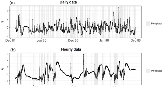
Figure 9.Time series ofηcorresponding to the parameter values at the maximum posterior density obtained with E1 in the Maimai catchment for daily and hourly resolution. Intervals whereP >0 are shaded in grey.

those problems are more related to τminthan to τmax, since higher values ofτmintend to coincide with bad performance. Or, in more general terms, the previously encountered prob-lems in the joint inference of hydrological and correlation parameters (Evin et al., 2013) seem to originate from pre-cipitation periods, not from dry periods. The fact that the in-ference ofτminis more successful in the Maimai catchment (Sect. 4.1.4), which has the simpler hydrological response, suggests that the realism of a hydrological model facilitates the successful inference of the correlation parameters.

These findings call for additional investigations into the is-sue of non-stationary correlation, potentially exploring other relationships betweenτ andP orQdet. Makingτ dependent onQdetinstead ofP would have the advantage that poten-tial low-pass filtering or time lag between precipitation and streamflow are taken care of by the hydrological model and need not be considered anymore in the error model. We per-formed some exploratory analysis in that direction, so far with limited success.

5.4 Shape of the distributionDQ

Relaxing the assumption of marginal normality ofQobsgiven

Qdet successfully reduced some very heavy outliers that strongly violated that assumption. However, this did not al-ways translate to improved distributional assumptions in the uniform space, where4reliis calculated. We suspect that the presence of strong outliers (large η) under the normal as-sumption led to the strong right-skew ofDQwhen inferring γ anddf, which was less appropriate for the rest of the dis-tribution of observed streamflows. In that case, a different distributional shape forDQwould be more appropriate, e.g.

a mixture distribution, which allows for some heavy tails on the upper side without skewing the central body too much to the right. Testing other distributional shapes for DQwas

beyond the scope of this study, however. Note that heavy outliers (i.e.η0) do not necessarily correspond to high streamflow; in both catchments the largestηwere observed during medium to low flows (Fig. 6a, b), namely during small peaks of observed streamflow that were not captured by the model.

The ranking in performance of the two options to either place the mean or the mode ofDQatQdet(Eq. 9) was dif-ferent for the two analysed catchments. The former led to better results in the Murg catchment, while the latter seemed preferable in the Maimai catchment. Ideally, we would like to satisfy both conditions, but this is obviously not possible whenDQis skewed.

Regarding the choice of the type of the distributionDQ,

recall thatQ(t )∼DQ(Qdet(t ),ψ). A distribution type with positive support would be a desirable alternative to the skewed Student’stdistribution, since it would ensure posi-tive streamflow without the need to assign the probability of

6 Conclusions

We presented and evaluated a flexible framework for proba-bilistic model formulations (i.e. likelihood functions) to de-scribe the total uncertainty of the output of deterministic hydrological models. This framework allows us to consider heteroscedastic errors with stationary correlation, non-equidistant observations and zero probability for negative streamflow. It does so by allowing for arbitrary and explicit marginal distributions for the observed streamflow at each point in time. For experts, it is easier to parameterise these marginal streamflow distributions than the distribution char-acterising the autoregressive model or some non-intuitive transformations like the Box–Cox transformation. The con-sistent implementation of this framework was successfully checked with a synthetic case study.

Using a simple deterministic hydrological bucket model and two case study catchments, the flexible framework was used to systematically test different error models on real-world data. Those error models represented various assump-tions about the statistical properties of the errors in terms of autocorrelation, skewness and kurtosis. The assumptions were found to have a profound effect on the quality of the predictions. The key findings are as follows:

1. We confirmed that, as shown in previous work by var-ious authors, accounting for autocorrelation with con-ventional approaches (represented by model E2) can lead to worse predictions than omitting autocorrelation (model E1). For example, model E2 had errors in cu-mulative streamflow of 76 % in the Murg catchment and 96 % in the Maimai catchment for hourly resolution in the calibration period. With model E1, in comparison, those errors were 1 % and 19 %, respectively. However, this result is unsatisfactory as there is clearly visible au-tocorrelation in the residuals that invalidates the model E1.

2. We showed that the predictions of conventional ap-proaches to deal with autocorrelation worsen signif-icantly as the temporal resolution increases. For ex-ample, the performance of model E2 in terms of the Nash–Sutcliffe efficiency decreases from 0.76 to 0.09 in the calibration period when moving from daily to hourly data resolution. In comparison, the performance of model E1 remains relatively stable (Nash–Sutcliffe efficiency decreases from 0.83 to 0.79).

3. Since rapid changes in a catchment’s storage change its memory, errors in streamflow are expected to show different correlations during precipitation events and dry weather. Based on the hypothesis that this non-stationarity increases when going from daily to hourly resolution, neglecting non-stationarity of correlation is the likely cause for finding 2.

4. Accounting for non-stationarity in autocorrelation sig-nificantly alleviated the observed problems of finding 2. In particular, allowing for the autocorrelation to be lower during wet than during dry periods (models E3 and E4) led to more stable behaviour across time res-olutions. For example, volume errors for model E3 in the Murg catchment were not larger that 3 % for all three investigated temporal resolutions. However, infer-ring the characteristic correlation time duinfer-ring precipita-tion events (model E3a) provided good results in only one of the two investigated catchments. Keeping that correlation fixed (model E3) could be seen as a prag-matic option with stable performance.

5. If the problems mentioned in finding 1 can be avoided, accounting for autocorrelation results in more realistic characteristics of model output than omitting autocorre-lation, which is confirming previous work. In particular, signatures such as the flashiness index are much bet-ter represented when including autocorrelation. For ex-ample, for an observed value of the flashiness index of 0.13 in the Maimai catchment in the calibration period, model E3a provided a value of 0.13, whereas model E1 resulted in a much larger value of 0.56.

6. Inferring the skewness and kurtosis of a skewed Stu-dent’stdistribution can lead to better-fulfilled distribu-tional assumptions about the errors. In our case study, this expectation was partly fulfilled for daily data, but not for data of higher frequency. For hourly data, for example, more freedom with respect to the shape of the distribution actually lead to less accurate representation of the observed distribution.

Appendix A: Derivation of the likelihood function To derive the conditional distribution ofQ(ti)|Q(ti−1)(and construct the likelihood function by iteratively multiplying the conditional probability densities), we have to propa-gate the distribution η(ti)|η(ti−1) given by Eq. (4) to the streamflow using the (inverse) transformationηtransgiven by Eq. (2).

In simplified notation (which makes it easier to get the key idea without getting in notational details), we get the follow-ing:

f Q(ti)|Q(ti−1)

=f η(ti)|η(ti−1)

dη(ti)

dQ(ti)

=

fOU η(ti)|η(ti−1)

fDQ Q(ti)

fN(0,1) η(ti)

, (A1)

where, in the final equation, fOU refers to the standard Ornstein–Uhlenbeck process defined by Eq. (4) and the ratio of the densitiesfDQ andfN(0,1) results from the derivative

and inner derivative of the transformation given by Eq. (2) (the derivative of cumulative distribution functions are the corresponding probability densities).

With explicit notation of functions and arguments, we get

f Q(ti)|Q(ti−1),θ,ψ

=fηtrans Q(ti), Qdet(ti,θ),ψ

|ηtrans Q(ti−1), Qdet(ti−1,θ),ψ

dηtrans

dQ Q(ti), Qdet(ti,θ),ψ

=f N

ηtrans Q(ti−1), Qdet(ti−1,θ),ψ

exp−ti−ti_τ−1

,

r

1−exp−2ti−ti−1

τ

ηtrans Q(ti), Qdet(ti,θ),ψ

·

f

DQ Qdet(ti,θ),ψ

Q(t_i)

fN(0,1)

ηtrans Q(ti), Qdet(ti,θ),ψ

. (A2)

This corresponds to the first sub-equation of Eq. (7). The or-der of the factors was changed in Eq. (7) to emphasise the product of the marginal distributionfDQwith a modification

Appendix B: Complete results

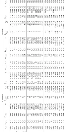
Table B1.Murg: summary of the predictions in the calibration and the validation period made with error models E1–E4 for different temporal resolutions of the hydrological data. Values are medians (and standard deviations) of the quality indices of the deterministic model output for the maximum posterior parameters, as well as those of 500 streamflow realisations produced with the full posterior parameter distributions. Recall that smaller values of4reliandspreadindicate better results.

∗_SmoothingP

err(t )with a moving-average window of size 5 h before applying Eq. (11).eDenotes the option where

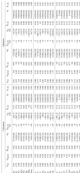
Table B2. Maimai: summary of the predictions in the calibration and the validation period made with error models E1–E4 for different temporal resolutions of the hydrological data. Values are medians (and standard deviation) of the quality indices of the deterministic model output for the maximum posterior parameters, as well as those of 500 streamflow realisations produced with the full posterior parameter distributions. Recall that smaller values of4reliandspreadindicate better results.

∗_{: smoothingP}

err(t )with a moving-average window of size 5 h before applying Eq. (11).e: denotes the option where