Mapping rainfall hazard based on rain gauge data: an objective cross validation framework for model selection

https://doi.org/10.5194/hess-23-829-2019 © Author(s) 2019. This work is distributed under the Creative Commons Attribution 4.0 License.

Mapping rainfall hazard based on rain gauge data: an objective

cross-validation framework for model selection

Juliette Blanchet1, Emmanuel Paquet2, Pradeebane Vaittinada Ayar1, and David Penot2 1_{Univ. Grenoble Alpes, CNRS, IGE, 38000 Grenoble, France}

2_{EDF – DTG, 21 Avenue de l’Europe, BP 41, 38040 Grenoble CEDEX 9, France} Correspondence:Juliette Blanchet ([email protected]) Received: 1 March 2018 – Discussion started: 23 March 2018

Revised: 23 January 2019 – Accepted: 5 February 2019 – Published: 13 February 2019

Abstract.We propose an objective framework for selecting rainfall hazard mapping models in a region starting from rain gauge data. Our methodology is based on the evaluation of several goodness-of-fit scores at regional scale in a cross-validation framework, allowing us to assess the goodness-of-fit of the rainfall cumulative distribution functions within the region but with a particular focus on their tail. Cross-validation is applied both to select the most appropriate sta-tistical distribution at station locations and to validate the mapping of these distributions. To illustrate the framework, we consider daily rainfall in the Ardèche catchment in the south of France, a 2260 km2catchment with strong inhomo-geneity in rainfall distribution. We compare several classical marginal distributions that are possibly mixed over seasons and weather patterns to account for the variety of climato-logical processes triggering precipitation, and several clas-sical mapping methods. Among those tested, results show a preference for a mixture of Gamma distribution over seasons and weather patterns, with parameters interpolated with thin plate spline across the region.

1 Introduction

In recent years, Mediterranean storms involving various spa-tial and temporal scales have hit many locations in south-ern Europe, causing casualties and damages (Ramos et al., 2005; Ruin et al., 2008; Ceresetti et al., 2012a). Assessing the frequency of occurrence of extreme rainfall in a region is usually done by the computation of return level maps. This requires relating any (large) amount of rainfall at a given lo-cation to its return level, i.e., to the frequency at which such

an amount is expected to occur on average at this location. In other words, it requires knowledge of the cumulative distri-bution function (CDF) of extreme rainfall at any grid point of the map. However, there are other situations when not only the largest rainfalls are of interest, but also smaller and even zero rainfall values. This is for example the case in rain-fall simulation frameworks, e.g., when rainrain-falls are input of spatially distributed hydrological models. In such a case one needs to be able to simulate any possible rainfall field. This implies knowing both the local occurrence of any rainfall value with the right frequency, and not only the largest ones, and their spatial co-occurrence. Other domains include the evaluation of numerical weather simulations (e.g., Froidurot et al., 2018) or the investigation of the climatology of rainfall events in a region.

inter-polation of point data supplied by rain gauges. This allows transformation of point observations into gridded ones, and so estimation of gridded CDFs of rainfall. Among the best performing methods for spatial interpolation of daily rain-fall are kriging, inverse distance weighting and spline-surface fitting (e.g., Camera et al., 2014; Creutin and Obled, 1982; Goovaerts, 2000; Ly et al., 2011; Rogelis and Werner, 2013). In complex topography, there may be some gain in applying these methods locally, e.g., considering local precipitation al-titude gradients (Frei and Schär, 1998; Gottardi et al., 2012; Lloyd, 2010). However, none of the above statistical methods is able to fully account for the statistical properties of rainfall fields. A first difficulty is due to the presence of zeros, which complicates interpolation and can lead to negative interpo-lated rainfalls – although this could be partially overcome by using analytical transformation of the raw variable. A second difficulty is that rainfall distribution is usually heavy tailed, and interpolation methods, by smoothing values, lack qual-ity for representing the most extreme events (Delrieu et al., 2014).

A second way of mapping rainfall hazard is, rather than in-terpolating the point observations, to map the parameters of CDFs fitted on rain gauge series. In addition to the choice of interpolation models comes now the choice of the marginal model of rainfall amounts on wet days (referred to as nonzero rainfalls). The most commonly used CDFs at daily scale in-clude the exponential, Gamma, lognormal, Pareto, Weibull and Kappa models (Papalexiou et al., 2013). Noting that these distributions tend to underestimate extreme rainfall amounts (Katz et al., 2002), a recent flurry of research de-veloped hybrid models based on mixtures of distributions for low and heavy amounts (Vrac and Naveau, 2007; Fur-rer and Katz, 2008; Li et al., 2012). More recently Naveau et al. (2016) proposed a family of distributions that is able to model the full spectrum of rainfall, while avoiding the use of mixtures of distributions. Several studies compared marginal models for rainfall (e.g., Mielke and Johnson, 1974; Swift and Schreuder, 1981; Cho et al., 2004; Husak et al., 2007; Papalexiou et al., 2013), but focusing usually on a couple of CDFs. Other studies compared methods for mapping rainfall hazard, and particularly extreme rainfall, assuming a given CDF (Beguería and Vicente-Serrano, 2006; Beguerïa et al., 2009; Szolgay et al., 2009; Blanchet and Lehning, 2010; Ceresetti et al., 2012b). However, there is, to the best of our knowledge, no study assessing the goodness-of-fit of the

fullprocedure of rainfall hazard mapping, i.e., from marginal modeling to the production of hazard maps.

Our study aims at filling this gap by proposing an ob-jective cross-validation framework that is able to validate the full procedure of rainfall hazard mapping starting from point observations. Our framework features three character-istics: (i) it selects both the marginal and mapping models, (ii) it validates the full spectrum of rainfall, from short- to long-term extrapolated amounts, and (iii) it applies on a re-gional scale. The framework is illustrated on the Ardèche

catchment in the south of France. Despite its relatively small size, this test case is particularly challenging as it shows ex-traordinarily strong inhomogeneity in rainfall statistics at a very short distance. Following previous studies in the region (Evin et al., 2016; Garavaglia et al., 2010, 2011; Gottardi et al., 2012), the compared marginal distributions involve seasonal and weather pattern subsampling, considering dif-ferent models for the subclass-dependent distributions. How-ever, the proposed cross-validation framework is general, as it involves objective criteria, and could likewise be used to select among any other distribution. Section 2 presents the data. Sections 3.1 and 3.2 describe the marginal distributions and mapping models considered in this study and present the cross-validation scores of model selection. Section 3.3 de-tails the procedure of model selection from marginal model-ing to hazard mappmodel-ing. Section 4 gives extensive results for the Ardèche catchment. Section 5 concludes the study.

2 Data

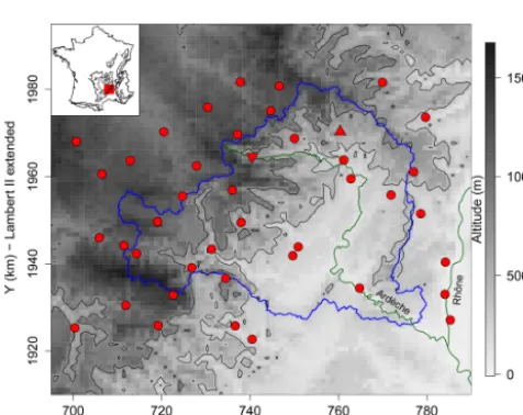
We illustrate our framework on the Ardèche catchment (2260 km2) located in the south of France (see Fig. 1). The region includes part of the southeastern edge of the Mas-sif Central, where the highest peaks of the region are lo-cated (more than 1500 m a.s.l), and the Rhône Valley (down to 10 m a.s.l). The southeastern slope of the Massif Central is known to experience most of the extreme storms and re-sulting flash floods (Fig. 2 of Nuissier et al., 2008). These so-called “Cévenol” events are produced by quasi-stationary mesoscale convective systems that stabilize over the region during several tens of hours. The positioning and stationar-ity of these systems are largely influenced by the topography of the surrounding mountain massifs (Nuissier et al., 2008). We use two daily rain gauge networks maintained, respec-tively, by Electricité de France and Météo-France. We con-sider the 15 rain gauges inside the catchment, together with the 27 stations located less than 15 km outside. This gives a total of 42 stations with 20 to 64 years of data between 1 Jan-uary 1948 and 31 December 2013. In both databases, daily values are recorded every day at 06:00 UTC, corresponding to rainfall accumulation between 06:00 UTC of the previous day and 06:00 UTC of the present day.

Table 1.Considered models for the marginal distributions of nonzero rainfall.0in the Gamma density is the complete Gamma function

0(κ)=

∞

R

0

rκ−1e−rdr.

Distribution CDFG(r)or densityg(r), forr >0 Parameters

Gamma g(r)=

rκ−1e−r/λ/ 0(κ)λκ

λ >0,κ >0

Weibull G(r)=1−e−(r/λ)κ λ >0,κ >0 Lognormal g(r)=expn−(log(r/λ))2/

2κ2

o /(rκ

√

2π ) λ >0,κ >0

Extended exponential G(r)=1−e−r/λκ λ >0,κ >0 Extended generalized Pareto G(r)=1−(1+ξ r/λ)−1/ξκ λ >0,κ >0,ξ >0

Figure 1. Region of analysis. The blue polygon is the Ardèche catchement. The red points show the locations of the stations. The upper triangle is station Antraigues and the lower triangle station Mayres (both lie at about 500 m a.s.l.). The background shows the altitude in gray scale (1 km raster cells). The top left insert shows a map of France with the studied region in red. The black lines are the 400 and 800 m a.s.l. isolines.

in the Massif Central plateau or in the Piémont. Concentra-tion of daily rainfall and particularly of extreme daily rainfall along the Massif Central ridge has already been documented in many studies; see, e.g., Fig. 10 of Blanchet et al. (2016). We assume in this study temporal stationarity of rainfall. A case of potential nonstationarity due to climate change will be discussed in Sect. 5.

3 Method

3.1 Marginal distribution of rainfall 3.1.1 Considered marginal models

Let R be the random variable of daily rainfall amount at a given station.Ris zero with probabilityp0and, for anyr >

0, we have the following decomposition:

pr(R≤r)=p0+1−p0G(r), (1) whereGis the CDF of nonzero rainfall at the considered sta-tion. Choice ofGis an issue. One of the difficulties is that we wish to model adequately both the bulk of the distribution of nonzero rainfall and its tail, i.e., the probability of extreme rainfall occurring. The most common models for nonzero rainfall include the Gamma, Weibull and lognormal mod-els (Papalexiou et al., 2013), whose CDFG(r)or densities g(r)=∂G(r)/∂r,r >0 are given in Table 1. Although less common, another family of models for nonzero rainfall relies on univariate extreme value theory, which tells that probabil-ities of the form pr(R≤r|r > q), withq large, can be ap-proximated by either an exponential or a generalized Pareto tail (Coles, 2001, Sect. 4). This led Naveau et al. (2016) to propose the extended exponential and extended generalized Pareto distributions, whose CDF is given in Table 1. Note that less parsimonious models are given in Naveau et al. (2016), but they are not considered in the present study. The extended exponential and extended generalized Pareto distri-butions of Table 1 ensure that the occurrence probability of small (but nonzero) rainfall amounts is driven byκ, while the upper tail of nonzero rainfall is equivalent to a generalized Pareto tail. The extended exponential model is also called “generalized exponential” and has been used previously for extreme rainfall in Madi and Raqab (2007) and Kazmierczak and Kotowski (2015).

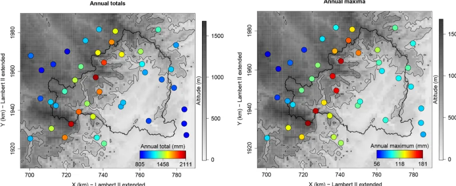
Figure 2.Panel(a): averages of annual totals (mm). Panel(b): averages of annual maximum daily rainfalls (mm).

is assigned to a WP. IfSseasons andKWP are considered, then days are classified into S×K subclasses. The law of total probability gives, for allr >0,

pr(R≤r)=

S

X

s=1 K

X

k=1

pr(R≤r|season=s,WP=k)ps,k, (2)

whereps,k is the probability that a given day is in seasons and in WP k (thusP

s

P

k

ps,k=1). Following Eq. (1),R in seasonsand WPkis zero with probabilityp0_s,kand, for any r >0, we have the decomposition

pr(R≤r|season=s,WP=k)=p_s,k0 +1−p_s,k0 Gs,k(r), whereGs,k is the CDF of nonzero rainfall at the considered station for a day in seasonsand WPk. This gives in Eq. (2), for allr >0,

pr(R≤r)=p0+

S

X

s=1 K

X

k=1 ps,k

1−p_s,k0 Gs,k(r), (3)

wherep0=

S

P

s=1 K

P

k=1

ps,kp0_s,kis the probability of any day be-ing dry. Nonzero precipitation amounts defined by Eq. (3) have CDF

G(r)=pr(R≤r|R >0)=

S

X

s=1 K

X

k=1

p0_s,kGs,k(r), (4)

where p0_s,k=ps,k(1−p_s,k0 )/(1−p0). Equation (4) defines a mixture of S×K distributions, e.g., a mixture ofS×K Gamma distributions. Analogously, the CDF of nonzero pre-cipitation amounts in a given seasonsis written as

Gs(r)=pr(R≤r|R >0,season=s)=

K

X

k=1

p00_s,kGs,k(r), (5)

wherep_s,k00 =ps,k(1−p_s,k0 )/(1− K

P

k=1

ps,kp_s,k0 ). A similar idea is used in Wilks (1998) for example, but considering a mix-ture of two (exponential) distributions in an unsupervised way, i.e., without relying on a priori subsampling. It shows the advantage of not requiring prior knowledge on the classi-fication, but it is at the same time more difficult to estimate, in particular if the models for different seasons and WP do not differ much.

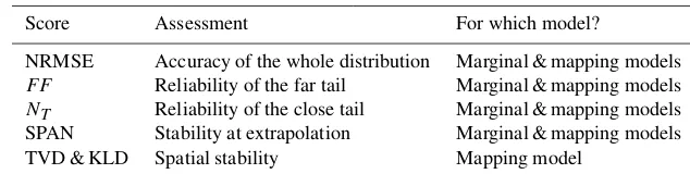
empiri-Table 2.Summary of the considered scores for evaluating marginal and mapping models.

Score Assessment For which model?

NRMSE Accuracy of the whole distribution Marginal & mapping models FF Reliability of the far tail Marginal & mapping models NT Reliability of the close tail Marginal & mapping models SPAN Stability at extrapolation Marginal & mapping models TVD & KLD Spatial stability Mapping model

cally aspˆ_s,k0 =d_s,k0 /d wheredis the number of observations andd_s,k0 is the number of zero values in seasonsand WPk. Combining estimations in Eq. (3) gives an estimation of the rainfall CDF at the considered station, and in Eq. (4) an esti-mation of the CDF of nonzero rainfall.

Estimates of return levels are then obtained as follows. The T-year return levelrT is the level expected to be exceeded on average once every T years. It satisfies the relationship pr(R≤rT|R >0)=1−1/(T δ), whereδis the mean number of nonzero rainfall per year at the considered station. When subsampling Eq. (4) is considered, there is no explicit for-mulation, and estimation of rT is obtained numerically by solving pr(R≤rT|R >0)=1−1/(T δ)in Eq. (4).

3.1.2 Evaluation at regional scale in a cross-validation framework

The goal of this evaluation is to assess which marginal model performs better at the regional scale, i.e., for a set ofn sta-tions taken as a whole, rather than individually. We follow the split sample evaluation proposed in Garavaglia et al. (2011) and Renard et al. (2013). We divide the data for each stationi into two subsamples, C_i(1) and C_i(2), and consider nonzero rainfall for these two subsamples. We fit a given competing model on each of the subsamples, giving two estimated dis-tributions ofGin Eq. (4):Gˆ(_i1), estimated onC_i(1), andGˆ(_i2), estimated onC_i(2). Our goal is to test the consistency between validation data and predictions of the estimates, both for the core and tail of the distributions, and the stability of the es-timates when calibration data changes, focusing particularly on the tail which is usually less stable.

As shown in Table 2, three families of scores are com-puted, assessing, respectively, (i) accuracy of the estima-tions along the full range of observaestima-tions (MEAN(NRMSE)), (ii) reliability of the tail of the estimated distribution, check-ing in particular systematic over- or under-estimation of the observations (AREA(FF) and AREA(NT)), and (iii) stabil-ity of the tail at extrapolation (MEAN(SPAN)). The scores relating the tail of the distribution have been proposed and used in Garavaglia et al. (2011), Renard et al. (2013) and Blanchet et al. (2015). In the split sample evaluation frame-work, four scores can be derived of a given score Sc: Sc(12)is the regional score whenG(_i2)is validated on the nonzero rain-fall subsample C_i(1). Sc(21), Sc(11) and Sc(22) are obtained

symmetrically. Sc(11)and Sc(22)are calibration scores, while Sc(12)and Sc(21) are cross-validation scores. For the sake of conciseness, we detail below the case of Sc(12)for the differ-ent scores.

The NRMSE (normalized root mean squared error) evalu-ates the reliability of the fits in the whole observed range of nonzero rainfall, by comparing observed and predicted return levels of daily rainfall. For a given stationi∈ {1, . . . ,Q},

NRMSE(_i12)=  

 1

n(_i1)

n(_i1)

X

k=1

r_i,T(1)

k− ˆr (2) i,Tk

2

 



1/2

, 1

n(_i1)

n(_i1)

X

k=1

r_i,T(1)

k, (6)

wheren(_i1)is the number of nonzero rainfall inC_i(1) for sta-tioni,Tkranges the observed return periods of nonzero rain-fall inC_i(1),r_i,T(1)

kis the observed daily rainfall associated with

the return periodTk for the subsampleC_i(1) andrˆ_i,T(2) k is the Tk-year return period derived from the estimatedGˆ(_i2). With-out loss of generality we assumeT1, . . . ,T_n(1)

i

to be sorted in descending order (soT1is associated with the maximum over C_i(1)). If stationi hasδi nonzero rainfall per year on average, usual practice is to consider thekth largest return period asTk=(n(i1)+1)/(δik),k=1, . . . ,n(i1), and to esti-mater_i,T(1)

kas thekth largest observed rainfall overC (1) i . Esti-materˆ_i,T(2)

k is obtained numerically from ˆ

G(_i2) as described in Sect. 3.1.1. The normalization by the mean rainfall ofC_i(1)in Eq. (6) allows comparison of NRMSE over stations with dif-ferent pluviometry. The smaller NRMSE(_i12), the betterGˆ(_i2) fits the rainfalls overC_i(1). For the set ofQstations, we ob-tain a vector of NRMSE(12) of length Qwhich should re-main reasonably close to zero. A regional score is obtained by computing the mean of theQvalues:

MEANNRMSE(12)= 1

Q Q

X

i=1

NRMSE(_i12). (7)

For competing models, the closer the mean is to 0, the better the goodness-of-fit.

NRMSE assesses goodness-of fit of the whole distribu-tion in the observed range. Now let us have a closer look at the tail of the distribution, and in particular at the maxi-mum overC_i(1); i.e., atr_i,T(1)

1 in Eq. (6), that for shortness we

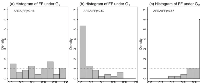
rain-Figure 3.Illustration of theFF score when the true CDFG0is extended exponential withλ=20 andκ=0.3. The CDFG1 underesti-mates G0 (λ=25) whileG2overestimatesG0(λ=15).(a)Histogram of{G0(m)}n wheremare 42 realizations ofGn₀ andn=4000.

(b)Histogram of{G1(m)}n.(c)Histogram of{G2(m)}n. The horizontal dashed lines show the uniform density on (0, 1).

fall, then the corresponding random variableM_i(1)has distri-bution Gi to the powern(i1), whose variance is large. Thus computing error based on the single realizationm(_i1) would be very uncertain. For this reason, Renard et al. (2013) pro-posed to make evaluation by pulling together the maxima of theQstations, after transformation to make them on the same scale. It is based on the idea that if X has CDF F, thenF (X)follows the uniform distribution on (0, 1). Taking X=M_i(1) andF =(Gi)n

(1)

i _{implies that, ifG}ˆ(2)

i is a perfect estimate ofGi, then

ff_i(12)= { ˆG(_i2)(m(_i1))}n(i1)

should be a realization of the uniform distribution. For the set ofQstations, this gives a uniform sampleff(12) of sizeQ. Hypothesis testing for assessing the validity of the uniform assumption is challenging because the ff_i(12) are not inde-pendent from site to site, due to the spatial dependence be-tween data. Thus Blanchet et al. (2015) proposed to base comparison on the divergence of the density of theff(12)to the uniform density. A reasonable estimate of the latter is ob-tained by computing the empirical histogram of the ff(12) with 10 equal bins between 0 and 1. As illustrated in Fig. 3, ifGˆ(_i2)are good estimates ofGi,i=1, . . . ,Q, the histogram offf(12)should be reasonably uniform on (0, 1). If the his-togram is left-skewed, thenGˆ(_i2)(m(_i1))tends to overestimate the trueG(_i1)(m(_i1)), or in other words the return period of the maximum overC_i(1)tends to be underestimated (case of over-estimated risk). If the histogram is right-skewed, the return period of the maximum overC_i(1)tends to be over-estimated (case of under-estimated risk). Although any scenario of mis-fitting could theoretically be possible, in practice the his-tograms offf(12)show mainly the three above alternatives: either a good fit (flat histogram), or a tendency towards a systematic under- or over-estimation (left- or right-skewed

histograms). By focusing of maximum values, the histogram offf(12)can be seen as a way of assessing systematic bias in the far tail of the distribution. For a more quantitative assess-ment, we compute the area between the density of theff(12) and the uniform density as follows:

AREAFF(12)= 1

18 10

X

c=1

10card(Bc) n −1

, (8)

where card(Bc)is the number offf_i(12) in thecth bin, for c=1, . . . , 10. The term inside the absolute value in Eq. (8) is the difference between densities in thecth bin. The division by 18 forces the score to lie in the range (0, 1), with lower values indicating better fits (the worst case being all values lying in the same bin). Figure 3 shows that, whenQ=42 stations are considered, a value of AREA(FF(12))around 0.2 corresponds to no systematic bias in the very tail of the dis-tribution at regional scale, whereas a value around 0.5 cor-responds to a strong over- or under-estimation. In the latter case, only looking at the histogram can inform about whether over- or under-estimation applies.

The NT criterion is an alternative to FF assessing re-liability of the fit of the tail but focusing on prescribed (large) quantiles rather than on the overall maximum. It applies the same principle as FF, involving a transforma-tion ofX toF (X), but considering X asK_i,T(1), the random variable of the number of exceedances over C(_i1) of theT -year return level, i.e., K_i,T(1)=card({Ri,j∈C_i(1); Gi(Rj) > 1−1/(T δi)}), in which case F is the binomial distribu-tion B_i(1) with parameters (n(_i1), 1/(T δi)). Thus, ifGˆ(_i2) is a perfect estimate ofGi, thenn(_i,T12)=B_i(1)(k(_i,T12)), where k(_i,T12)=cardnri,j∈Ci(1); ˆG

(2)

i lef t (ri,j

>1−1/ (δiT )}

,

variate on (0, 1) is proposed in Renard et al. (2013) and exten-sively described in Blanchet et al. (2015). Foriranging over the set ofQstations, we thus obtain a sample ofQuniform variates. Scores are calculated as for FF by comparing the empirical densities ofN_T(12) to the theoretical uniform den-sity, giving the scores AREA(N_T(12)). TakingT as, e.g., half to one-quarter the length of the observations allows assess-ment of the reliability of the close tail of the distribution. As such, it is a good complement toFF that focuses on the far tail (i.e., on the maximum).

Last but not least, the SPAN criterion evaluates the stabil-ity of the return level estimation, when using data for each of the two subsamples. More precisely, for a given return pe-riodT and stationi,

SPANi,T =

| ˆr_i,T(1)− ˆr_i,T(2)|

1/2nrˆ_i,T(1)+ ˆr_i,T(2)o

, (9)

whererˆ_i,T(1); e.g., is theT-year return level for the distribu-tion G estimated on subsampleC_i(1) of station i, i.e., such thatGˆ(_i1){ ˆr_i,T(1)} =1−1/(T δi). SPANi,T is the relative abso-lute difference inT-year return levels estimated on the two subsamples. It ranges between 0 and 2; the closer to 0, the more stable the estimations for stationi. For the set ofQ sta-tions, we obtain a vector of SPANT of lengthQwith a dis-tribution which should remain reasonably close to zero. A rough summary of this information is obtained by comput-ing the mean of theQvalues of SPANi,T,i=1, . . . ,Q:

MEAN(SPANT)= 1 Q

Q

X

i=1

SPANi,T. (10)

For competing models, the closer the mean is to 0, the more stable the model is. When T is larger than the observed range of return periods, MEAN(SPANT) evaluates the sta-bility of the return levels in extrapolation. Note that it is by definition 0 in calibration, and thus it is only useful in cross-validation.

For the sake of concision, in the rest of this article the scores MEAN(NRMSE), AREA(FF), AREA(NT) and MEAN(SPANT) will be referred to as the NRMSE,FF,NT and SPANT scores.

3.2 Mapping of the margins 3.2.1 Considered mapping models

LetRi be the random variable of daily rainfall at stationi, i=1, . . . ,Q. Applying Sect. 3.1 at stationi gives an esti-mateGˆi(r)of the CDFGi(r)=pr(Ri≤r|Ri>0). Our goal is to derive an estimate of the CDF of nonzero daily rainfall at any locationlof the region, pr(R(l)≤r|R(l) >0), based on theQestimated CDFsGˆi(r). Locationlrefers here to the three coordinates of ground projection coordinates and alti-tude, that we writel=(x,y,z). Letθˆibe the set of estimated

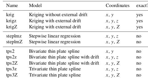
Table 3.Mapping models considered in this study, with involved coordinates. Kriging method provides exact interpolation, unlike the linear regression and thin plate spline.

Name Model Coordinates exact?

krig Kriging without external drift x,y yes krigz Kriging with external drift x,y,z yes krigZ Kriging with external drift x,y,Z yes steplmz Stepwise linear regression x,y,z no steplmZ Stepwise linear regression x,y,Z no

tps2 Bivariate thin plate spline x,y no tps2z Bivariate thin plate spline with drift x,y,z no tps2Z Bivariate thin plate spline with drift x,y,Z no tps3z Trivariate thin plate spline x,y,z no tps3Z Trivariate thin plate spline x,y,Z no

parameters for stationi andθˆi,j itsjth element.θˆi is com-posed of theS×Kprobability of zero rainfallp0_s,k and the 2×S×Kor 3×S×Kparameters of the distributionsGs,k, depending on the marginal distribution (see Table 1). We as-sume theθi,j ordered so that the first S×K elements are the p_s,k0 . We aim at estimating the surface response θj(l) at anyl of the region, knowing θj(li)= ˆθi,j. In this study we consider three of the most popular method: kriging in-terpolation, linear regression methods and thin plate spline regressions. However, the parameters θjs are constrained, whereas these models apply the unbounded variables: the probabilitiesp0_s,k lie in (0, 1), while the parameters of Ta-ble 1 are all positive. Therefore we apply the mapping mod-els to transformations ofθj, i.e., toψj=transf(θj), where “transf” maps the range of values ofθj to (−∞, +∞). In this study we considerψj(l)=8{θj(l)}ifj ≤S×K(i.e., if θjis anyp0s,k), where8is the standard Gaussian CDF, and to ψj(l)=log{θj(l)}otherwise. Other transformations would be possible, in particularp_s,k0 may be transformed with the logit function, but will not be considered here for the sake of concision. Thus we aim at estimating ψej(l) given val-ues ψj(li)= ˆψi,j at station locations, with obvious nota-tions. Ifl≤S×K, estimates of θj(l)are then obtained as

eθj(l)=8−1(ψej(l)). Otherwise surface response estimates are obtained aseθj(l)=exp(ψej(l)). For the sake of clarity, we omit below the indexj, considering a surfaceψ (l)to be estimated for alllin the region, given valuesψ (li)= ˆψi.

The considered mapping models are listed in Table 3. Three families of method are considered: kriging, linear re-gression and thin plate spline. Additionally to how they map values, there is a fundamental difference between these mod-els: kriging is an exact interpolation, i.e.,ψ (le i)= ˆψi at any station locationliused to estimate the model. By contrast, the linear regression models and thin plate splines provide inex-act interpolations: in the great majority of the time,ψ (le i)6=

ˆ

The external drift, if any, is modeled as a linear function of altitude (i.e., of the forma0+a1ζ), consideringζas either the altitude of the station (z) or, following Hutchinson, 1998, as a smoothed altitude (Z) derived by smoothing a 1 km digital el-evation model (DEM) with 5 km moving windows (i.e., tak-ingZas the average altitude of 25 DEM grid points). The re-sults that will be presented below correspond to the case of an exponential covariance function of the form ρ(h)=e−h/β, withβ >0. We also considered the case of a powered expo-nential covariance functionρ(h)=e−(h/β)ν with 0< ν≤2, but this resulted in a slight loss of stability due to the ad-ditional degree of freedom, without improving the accuracy at regional scale. For the sake of concision, these results are not presented here. Combining alternatives for the drift part gives a total of three kriging interpolation models with two to three unknown parameters each, for eachψ. Estimations of the kriging models are made by maximizing the likelihood associated with the_ψiˆ _{, assuming thatψ (l)is a Gaussian}

pro-cess (see Sect. 5.4 of Diggle and Ribeiro, 2007). Alterna-tives are to estimate drifts and variograms by least squares in different steps, with the risk of biasing estimates (Sect. 5.1 to 5.3 of Diggle and Ribeiro, 2007). Both estimation meth-ods are available in R package “geoR” (e.g., functions “lik-fit” and “vario“lik-fit”). In the case without drift, prediction at any sitelof the region is obtained as

e

ψ (l)=

Q

X

i=1

wi(hi)ψˆi, (11)

where the weightswi(hi)are derived from the kriging equa-tions and satisfy

Q

P

i=1

wi(hi)=1. The weights depend on the estimated covariance function and on the distance hi be-tweenland station locationli in the (x,y) space (i.e.,h2i = (x−xi)2+(y−yi)2). In the case with external drift, predic-tion at any locapredic-tionlof the region is then obtained as

e

ψ (l)=a1ζ+ Q

X

i=1 wi(hi)

ˆ

ψi−a1ζi

, (12)

whereζ is the altitude at locationl(i.e., eitherzorZ). Pre-dictions (Eqs. 11 and 12) are exact:ψ (le i)= ˆψi, and conse-quentlyeθ (li)= ˆθi.

For the linear regression models, we start from regres-sions of the formψ (l)=a0+a1x+a2y+a3ζ+a4x2+a5y2+ a6xy+a7xζ+a8yζ+(l), where(l)∼N (0,σ2)andζis, as before, either the altitude of the station (z) or the smoothed altitude (Z). We consider the Akaike information criterion (AIC), defined as AIC=2η−2 logL, whereηis the num-ber of parameters (10 at the start) and L is the maximum likelihood value of the regression model. The lower AIC, the better the model. Then we repeatedly drop the variable that increases most the AIC – if any –, and add the variable that decreases most the AIC – if any. This stepwise method is implemented in the “step” function of R package “stats”. At

algorithm stop, the model may contain 1 to 10 parameters, for each ψ. Predictionseθ (l) are then obtained as the back

transformation of the estimated regressions.

Last but not least, bivariate and trivariate thin plate splines are considered for ψ (l) (Boer et al., 2001; Hutchinson, 1998). These methods are implemented in function “Tps” of R package “fields”. In the bivariate case,ψ (l) is modeled asψ (l)=u(x, y)+(x, y), whereuis an unknown smooth function and(x, y)are uncorrelated errors with zero means and equal variances. The functionuis estimated by minimiz-ing

Q

X

i=1

ˆ

ψi−u (xi, yi)

2 +λ +∞ Z −∞ +∞ Z −∞ (

_∂2_{u(x, y)} ∂x2

2

+2

_∂2_{u(x, y)}

∂x∂y

2

+

_∂2_{u(x, y)}

∂y2

2)

dxdy, (13)

whereλis the so-called smoothing parameter, which controls the trade-off between smoothness of the estimated function and its fidelity to the observations. It can be estimated by generalized cross-validation. Then predictions are obtained as

e

ψ (l)=a0+a1x+a2y+ Q

X

i=1

bih2ilog(hi) , (14)

wherehi is the Euclidean distance in the (x,y) space be-tweenland station locationli. The partial trivariate case as-sumes thatψ (l)−a3ζ is a bivariate thin plate spline, where a3is fixed andζis eitherzorZ. To make the connection with kriging,ψ (l)can thus also be seen as a bivariate thin plate spline with (fixed) drift inζ. The coefficienta3is estimated in a preliminary step by regressingψˆi againstζi. Estimation of the bivariate thin plate spline forψ (l)−a3ζis made as de-scribed above given the values ofψˆi−a3ζi. Predictions are obtained as

e

ψ (l)=a0+a1x+a2y+a3ζ+ Q

X

i=1

bih2_ilog(hi) . (15)

Finally in the trivariate case, we have ψ (l)=u(x, y, ζ )+

(x, y, ζ ). The minimization problem is similar to Eq. (13) with a penalization enlarged by several terms (Wahba and Wendelberger, 1980). Predictions are then obtained as

e

ψ (l)=a0+a1x+a2y+a3ζ+ Q

X

i=1

bih0i, (16)

Note that the trivariate case (Eq. 16) differs from the bivariate case with drift (Eq. 15) in two ways. First, Eq. (16) considers distance in the (x,y,ζ) space, whereas Eq. (15) considers distance in the (x,y) space. Second, in Eq. (16), the weights associated with the stations are linear functions of the dis-tance, unlike in Eq. (15) (see the termh2_ilog(hi)vs.h0_i). 3.2.2 Evaluation at regional scale in a cross-validation

framework

Evaluation is performed in two ways. The first one is a leave-one-out cross-validation scheme aiming to test at regional scale how the interpolated distributions are able to fit the data of the stations when these data are left out for estimating the mapping model. The second step assesses spatial stabil-ity by comparing the interpolated distributions obtained at a given station whether the data of this station are used or not in the mapping estimation. In other words, it is a comparison between leave-one-out and leave-zero-out mappings. So the two evaluations differ in that the first one compares an inter-polated distribution to data, while the second step compares two interpolated distributions.

First, let us consider a given parameter estimate θˆ_i,j(1) obtained at station i based on the subsample C_i(1) (for a given marginal model). We apply a leave-one-out cross-validation scheme: for each stationi0 alternatively, we use the set of θˆ_i,j(1), i6=i0 to estimate the surface response

e

θ_j(1)(l). We store the value of this estimate at station loca-tioni0, i.e.,eθ

(1)

j (li0)=eθ

(1)

i0,j. Repeating this for every

param-eter θj gives an estimation of the full set of parameters at stationi0, i.e., estimationGe

(1)

i0 ofGi0. Iterating over the

sta-tions, we obtain new estimatesGe

(1) 1 , . . . ,Ge

(1)

Q ofG1, . . . ,GQ. Applying similarly for the subsample C_i(2) gives estimates

e

G(₁2), . . . ,Ge

(2)

Q. We can assess the reliability of these esti-mates at the regional scale by computing the scores Sc(11), Sc(22), Sc(12)and Sc(21)of Sect. 3.1.2, whereGiˆ is replaced byGie. Note that all these scores are cross-validation scores

since the estimatesGe

(1) 1 andGe

(2)

1 are computed without us-ing any data of stationi.

Second, we consider the set of all θˆ_i,j(1), i=1, . . . ,Q to estimate the surface responseeθ

(1)

j (l). We store the value of this function at every station location, giving new estimates

e

G∗₁(1), . . . ,Ge

∗(1)

Q . Note that in the particular case of kriging,

e

G∗_i(1)is exactlyGˆ(_i1)since it is an exact interpolation method, so everyθˆ_i,j(1)equalseθ

∗(1)

i,j . We can assess the stability of the interpolated distributions at a given location li when obser-vations are available or not at this location by comparing

e

G∗_i(1)(r) andGe

(1)

i (r)for allr. For this we discretizer be-tween 0 and 450 mm (which is the overall maximum rain-fall) with 1 mm step and we compute the total variation dis-tance (TVD) between Ge

∗(1) i and Ge

(1)

i and the Kullback– Leibler divergence (KLD, Weijs et al., 2010) from Ge

∗(1) i

toGe

(1)

i , which are given by TVD(_i1)=sup

r

|Ge

∗(1) i (r)−Ge

(1) i (r)|,

KLD(_i1)= Z

r

e

g_i∗(1)(r)logeg

∗(1) i (r)

eg

(1) i (r)

dr,

where, e.g.,_eg_i(1)is the density function associated withGe

(1) i . Note that the KLD is not symmetric. Written as such, it can be interpreted as the amount of information lost when

e

G(_i1) is used to approximateGe

∗(1)

i , so consideringGe

∗(1) i as the “true” distribution of data. TVD and KLD differ in that TVD focuses on the largest deviation between the two CDFs, whereas KLD somewhat integrates deviations along rain-falls. Obviously, one would like the interpolation to be as stable as possible when data are available or not at stationi, i.e., that the lower TVDi and KLDi, the more stable the in-terpolation at stationi.

Regional scores MEAN(TVD(_i1)) and MEAN(KLD(_i1)) are then obtained by computing the mean of the Q values. MEAN(TVD(_i2)) and MEAN(KLD(_i2)) are obtained similarly for the subsample C(2). For competing models, the closer the means are to 0, the more spatially stable is the inter-polation. For shortness, we will refer to MEAN(TVD) and MEAN(KLD) as the TVD and KLD scores, respectively (Ta-ble 2).

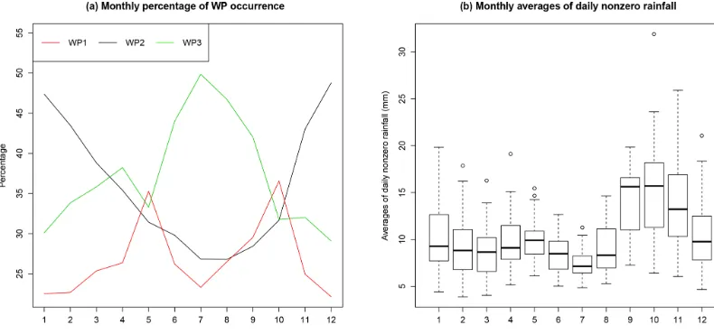
Figure 4. (a) Monthly percentage of occurrence of the three WPs.(b) Boxplot of the monthly averages of daily nonzero rainfall. Each boxplot contains 42 points (one point per station).

In cases where subsampling is also undertaken by season, we impose a restriction of S being two seasons, represent-ing the season-at-risk durrepresent-ing which most of the annual max-ima are observed, and the season-not-at-risk. Furthermore, we impose the season-at-risk to be the same for all the sta-tions due to the little extent of the region. Based on Fig. 4, we define the season-at-risk as the three months of September, October and November, as in Garavaglia et al. (2010) and Evin et al. (2016) for example. Alternative for bigger regions would be to select the months composing the season-at-risk following the procedure described in Blanchet et al. (2015). 3.3.1 Marginal selection procedure

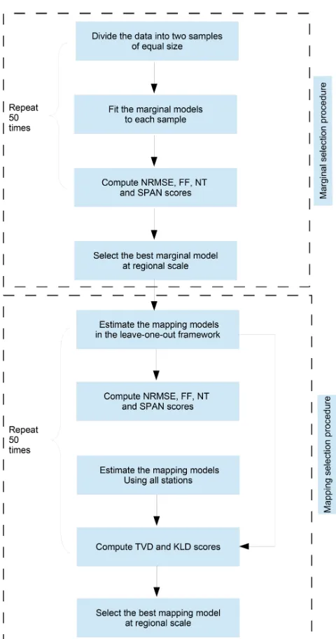
The full cross-validation procedure for selecting both the marginal and mapping models is summarized in Fig. 5. First we consider the marginal distributions of Table 1 and select the best of them at regional scale, as described in Sect. 3.1.2: 1. We divide the days of 1948-2013 into two subsamples of equal size, denoted C(1) andC(2). Given the weak temporal dependence of rainfall in the region (80 % of the wet periods have length lower than 3), division is made by randomly choosing blocks of five consecutive days to compose C(1), the remaining blocks compos-ingC(2).

2. For every stationi, we consider the set of observed days inC(1)andC(2), givingC_i(1)andC(_i2).

3. We fit each distribution of Table 1 to the two subsam-ples, getting estimates Gˆ(_i1) andGˆ(_i2) of each distribu-tion and for every stadistribu-tion.

4. We compute the scores of Sect. 3.1.2, getting two cal-ibration scores – (11) and (22) – of NRMSE,FF and

NT, and two cross-validation scores – (12) and (21) – of NRMSE,FF,NT and SPANT. ForNT, we consider T =5 years, which is lower than the minimum length of the calibration data and allows one to focus on the tail but still have several exceedances of theT-year return level at every station. SoFF, by focusing on the maxi-mum of roughly 10 to 30 years of data, can be seen as an evaluation score for the far tail, whileN5can be seen as an evaluation score for the close tail. For SPANT, we considerT =100 andT =1000 years in order to test extrapolation far in the tail but at a scale still commonly used for engineering purposes (dam building, protec-tions, etc., Paquet et al., 2013).

5. We repeat 50 times steps 1–4.

We obtain 100 values of each calibration score and 100 val-ues of each cross-validation score. We apply this procedure to the four distributions of Table 1, considering the four al-ternatives: no season nor WP (S=1, K=1), two seasons but no WP (S=2,K=1), no season but three WPs (S=1, K=3), two seasons and three WPs (S=2,K=3). Com-paring the distributions of the scores of the 16 models allows us the select the marginal distribution yielding to the best fit at regional scale. We select this marginal model for further consideration.

3.3.2 Mapping selection procedure

Second we consider the mapping models of Sect. 3.2.1 for interpolating the selected marginal model, and we select the best of them in two ways, as described in Sect. 3.2.2.

1. We consider the estimatesGˆ(_i1,t ),i=1, . . . ,Q, obtained at the tth iteration of the marginal selection proce-dure, and corresponding to the subsamplesC_i(1,t ),i=

Figure 5.Schematic summary of the full cross-validation procedure for selecting both the marginal and mapping models.

2. We estimate the mapping models of Sect. 3.2.1 fol-lowing the leave-one-out cross-validation framework of Sect. 3.2.2. We obtain new estimatesGe

(1,t )

i for each sta-tioniand each mapping model. EachGe

(1,t )

i is a cross-validation estimation of both G(_i1) andG(_i2) since the computation ofGe

(1,t )

i did not use any data of stationi. 3. We compute the scores of Sect. 3.1.2 associated with

e

G(_i1,t ),i=1, . . . ,Q. We obtain for each score two val-ues (e.g., FF(11) andFF(21) when consideringGe

(1,t ) i and the maximum value over either C(1) or C(2)). All these scores are cross-validation scores.

4. We estimate the mapping models of Sect. 3.2.1, using all the stations to make interpolation. We obtain new estimatesGe

∗(1,t )

i for each stationi and each mapping model.

5. We compute the spatial means of the TVD and KLD scores of Sect. 3.2.2, comparingGe

∗(1,t ) i to Ge

(1,t ) i , for, i=1, . . . ,Q.

6. We repeat steps 1–5 for the estimatesGe

(2,t )

i correspond-ing to the subsampleC_i(2,t ).

7. We repeat steps 1–6 for each of the 50 subsamples. We obtain 200 values of each cross-validation score NRMSE,FF,NT and SPAN, and 100 values of the TVD and KLD scores. Comparing the distributions of these scores allows us the select the mapping model yielding the smallest score, for the selected marginal model. We select this map-ping model for further consideration.

At this step we have selected the best marginal model and the best mapping model (among those tested) for our data. 3.3.3 Final regional model

Finally, we consider the whole sample of data and apply the selected marginal distribution and mapping model.

1. We estimate the selected marginal distributionGˆ∗_i based on the full data, giving parametersθˆ_ij∗,i=1, . . . ,Q. 2. We estimate the mapping model associated with each

marginal parameter, using allθˆ_ij∗,i=1, . . . ,Q, to esti-mate the surface responseeθ_j∗(l).

We obtain estimates of pr(R(l)≤r|R(l) >0) for every lwithin the region, making full use of the observations. Es-timation of pr(R(l)≤r)is obtained straightforwardly from Eq. (3). Although not considered in this study, confidence in-tervals could be obtained by bootstrapping within these two last steps.

4 Results

4.1 Selection of the marginal distribution

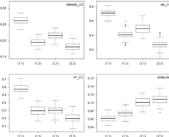
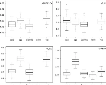
Figure 6.Scores of cross-validation whenGs,kare Gamma distributions and the number of seasons and WP varies:S∈ {1, 2}andK∈ {1, 3}. The values of (S,K) are indicated in thexlabels. Each boxplot contains 100 points.

forT =1000 years lead to the same conclusions (correlation 99.9 % between SPAN100and SPAN1000).

Comparing the reliability scores NRMSE, FF and N5when neither season nor WP is used – case (1, 1) – with cases when either WPs – case (1, 3) – or seasons (case (2, 1)) are considered shows there is at regional scale a clear im-provement in using a mixture of Gamma distributions rather than considering a single Gamma for the whole year. Reli-ability criteria are slightly better (i.e., lower) when WPs are considered rather than season, but this is more marked for the bulk of the distribution (represented by the NRMSE scores) than for its tail (FF andN5). Reliability scores are even bet-ter when both seasons and WPs are considered – case (2, 3) –, particularly for the tail of the distribution.

Obviously, there is a loss of stability when considering seasons and/or WPs due to the increased number of param-eters. However, the score of SPAN100 ranges from 0.08 to 0.14, which means that the two estimates of the 100-year re-turn levels overC(1) andC(2) differ by 8 % to 14 %, which seems acceptable.

We illustrate the quality of the fit for station Antraigues, located in the very foothills of the Massif Central slope (see Fig. 1), which shows among the largest annual maxima (see Fig. 2). We focus on the tail of the distribution by looking at the return level plot (here beyond the yearly return period). Of course, some variability is found in the return level es-timations depending on the subsample used for estimation.

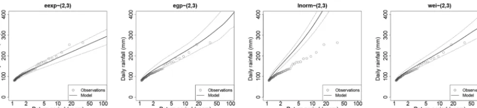
Figure 7 illustrates this by showing the 95 % envelope of re-turn level estimations over the 100 subsamples on eitherC(1) orC(2) together with the full sample of 35 years. Note that the envelopes do not show confidence intervals (that could be obtained by bootstrapping for example), but variability when only half the data are used from calibration. Thus, more than goodness-of-fit assessment, the plots of Fig. 7 al-low us to assess the quality of the fits at close extrapolation (i.e., when extrapolating at twice the length of the data). The plots clearly show that considering seasons and WPs allows us to get heavier-tailed distributions. The median estimates with two seasons and three WPs follow most closely the em-pirical points, even the largest ones, showing the quality of the fits for extrapolating at twice the length of the data. How-ever, we note that the return level plots of Fig. 7 all appear approximately linear for high values, meaning that none of the Gamma mixtures is able to produce heavy tails in the sense of extreme value theory. It is possible that return levels at extrapolation far beyond the observed return periods are underestimated. Figure 7 also shows that variability is rel-atively low in all cases, although it naturally increases for the marginal models involving more parameters. In particu-lar, the coefficient of variation of the 100-year return level with two seasons and three WPs is less than 7 %, in coher-ence with the SPAN100of Fig. 6 at regional scale.

mix-Figure 7.Case of Antraigues whenGs,kare Gamma distributions and the number of seasons and WP varies:S∈ {1, 2}andK∈ {1, 3}. The values of (S,K) are indicated in the title. The dotted lines show the 95 % envelope of return level estimates over the 100 subsamples. The plain line shows the median estimates. The gray points show the full sample (35 years). Each estimation is based on half of these points.

Figure 8. Scores of cross-validation when Gs,k is either the extended exponential (eexp), extended generalized Pareto (egp), Gamma (gamma), lognormal (lnorm) or Weibull (wei) distribution, withS=2 andK=3. Each boxplot contains 100 points. The boxplots of reliability scores in the lognormal case are missing because they lie far above the upper range of depicted values.

ture model withS=2 seasons andK=3 WPs for further investigation. Figure 8 shows the scores of cross-validation when the parent distributionGs,kis either the extended expo-nential, extended generalized Pareto, Gamma, lognormal or Weibull distribution. The reliability scores NRMSE,FF and N5 in the lognormal case are missing because they lie far above the upper range of the depicted values (e.g., the me-dian NRMSE is about 0.7), which clearly rules out the use of the lognormal model for this region. The reliability criteria of the four other distributions all show the same pattern: a better performance of the Gamma model, closely followed by the extended exponential case. Then comes the extended

Figure 9.Case of Antraigues whenGs,kis either the extended exponential (eexp), extended generalized Pareto (egp), lognormal (lnorm) or Weibull (wei) distribution, withS=2 andK=3. The dotted lines show the 95 % envelope of return level estimates over the 100 subsamples. The plain line shows the median estimates. The gray points show the full sample (35 years). Each estimation is based on half these points. The case of the Gamma distribution is shown in panel(d)of Fig. 7.

generalized Pareto distribution on the upper tail of the data (not shown).

Stability score SPAN100 in Fig. 8 shows that the most stable model is the lognormal case, but this is because the lognormal distribution gives unreasonably huge estimates of large return values (as illustrated in Fig. 9 for station Antraigues, for example), giving very large normalization terms in the SPAN criteria (see Eq. 9). The fact that the lognormal model has by far the worst reliability scores but the best stability score preaches for the conjoint use of these two families of scores not to misinterpret results. The stabil-ities of the Gamma and extended exponential distributions are very similar and fairly less good than the lognormal case. Then comes the Weibull distribution, and finally the general-ized Pareto distribution, which is clearly the least stable.

Figure 9 illustrates the quality and spread of the fits de-pending on the distribution for station Antraigues, when es-timation is made on either subsample. Compared to Fig. 7, it confirms that the Gamma and extended exponential mod-els perform almost alike. Median estimations differ by about 5 % for the 100-year return level (303 mm for the Gamma vs. 287 mm for the extended exponential model) and by about 7 % for the 1000-year return level (414 mm vs. 386 mm), with very similar widths of the 95 % envelopes (e.g.,±40 mm for the 100-year return level). The lognormal model clearly fails to reproduce return periods larger than 1 year, giving much too heavy tails despite a reasonably good fit of the bulk. Actually the skewness – which informs some-how about the “ asymmetry of the bulk” – is reasonably well estimated, whereas the kurtosis – which informs about the heaviness of the tail – is much overestimated. This is in line with Fig. 2 of Hanson and Vogel (2008), which shows that when the skewness of daily rainfall across the US is well estimated by the lognormal distribution, then the kurtosis is much overestimated. Note that Papalexiou et al. (2013) did not find such ill-fitted tails with the lognormal distribution, but in their case fitting is made on the tail (i.e., on the largest values), whereas the lognormal model seems to fail when ad-justing both the bulk and the tail of rainfall distribution. The

Weibull and extended generalized Pareto models give very similar fits up to the 50-year return period, but the return level plot of the extended generalized Pareto model is more con-vex (i.e., it shows a heavier tail) than for the Weibull model, giving a median estimation 8 % larger for the 100-year return level (390 mm vs. 358 mm) and 35 % larger for the 1000-year return level (799 mm vs. 522 mm). The width of the 95 % en-velope is also larger in both absolute and relative values, in coherence with the SPAN100 of Fig. 8 at regional scale. Fi-nally, both the Weibull and extended generalized Pareto mod-els overestimate the return levmod-els associated with 1–5 years, unlike the Gamma and extended exponential models. This tendency towards overestimation of the tail is actually a quite general feature observed for most the stations, giving too fre-quently low values offfi andni,T, as already stated.

The results of Figs. 8 and 9 lead us to conclude that the best performance for the region is achieved by the Gamma and extended exponential models, which actually perform very similarly for Antraigues station. Note that exactly the same conclusions hold when focusing on the season-at-risk rather than considering the whole year, i.e., when computing the cross-validation scores for the estimated seasonal distri-butionGsin (5) rather than for the year-round distributionG in Eq. (4. Due to its slightly better performance at regional scale for adjusting the tail of the distribution (FF andN5in Fig. 8), we select the Gamma model (with two seasons and three WPs) for further consideration.

4.2 Selection of the mapping model

Figure 10. Scores of mapping whenGs,k are Gamma distributions withS=2 and K=3 whose parameters are interpolated with the mapping models of Table 3. The first two rows show leave-one-out cross-validation scores. Each boxplot contains 200 points. The third row compares interpolations at a given station whether the data of this station are used or not in the interpolation. Each boxplot contains 100 points.

any mapping gives less accurate estimations of the full dis-tributions than the local fits. Loss in accuracy is equivalent and relatively small for all kriging interpolations and the bi-variate thin plate splines (with or without drift), while the trivariate thin plate spline and even more the linear model are less accurate. A closer look at the fits of all stations reveals that the strong loss in NRMSE for these two methods is ac-tually due to a few stations that are systematically very badly

Figure 11.Cases of Antraigues (panelsa–d) and Mayres (panelse–h) whenGs,kare Gamma distributions withS=2 andK=3 whose parameters are interpolated with either kriging without external drift (krig), a stepwise linear model (steplmZ), a bivariate thin plate spline with drift (tps2Z), or a trivariate thin plate spline (tps3Z). The dotted lines show the 95 % envelope of return level estimates over the 100 subsamples. The plain line shows the median estimates. In black, each interpolation is based on half the data of the other stations, excluding the considered station. In red, interpolation is based on half the data of all the stations, including the considered station. The gray points show the full sample (35 years for both stations).

Back to the kriging methods, the three tested alternatives give very similar fits, with slightly less stability when con-sidering a drift in station altitude z, while considering the smoothed altitudeZis useless becausea1in Eq. (12) is al-most always zero. The best kriging method for our region study in thus the simple kriging interpolation. This method is only slightly beaten in accuracy by the bivariate thin plate spline (with or without drift), but which is slightly less sta-ble. However, the TVD and KLD scores comparing the spa-tial stability of the mappings show that the bivariate thin plate splines are clearly more stable in space than all krig-ing methods. The linear model is even more stable but, as al-ready said, it is much less accurate. Finally, comparing the five cases of thin plate spline shows that the three bivari-ate cases clearly outperform the trivaribivari-ate case, both in terms of accuracy and stability. Comparing the bivariate case with drift (Eq. 15) to the the trivariate case (Eq. 16) shows the usefulness of considering nonlinear weights of the distance (through the termh2_ilog(hi)vs.h0_i). Last but not least, what-ever the method but particularly for the thin plate spline, bet-ter accuracy and stability is achieved when the smoothed alti-tudeZis considered rather than the station altitudez, as also found in Hutchinson (1998) for interpolating rainfall data.

We illustrate the results in Fig. 11 for the Antraigues sta-tion, adding to that the case of the worst fit of the thin plate spline, which is for the station of Mayres. Mayres lies at about 500 m a.s.l., as does Antraigues, but it is located at the

Figure 12.Map of the probability of daily rainfall exceeding 1 mm and of the mean of nonzero rainfall in the three WPs of the season-at-risk. The points are colored with respect to the empirical estimates.

We conclude following the results of Figs. 10 and 11 that the best interpolation method (among those tested) is the bi-variate thin plate spline with drift in smoothed altitude, which is slightly more accurate but much more spatially stable than the kriging method. The trivariate thin plate spline and the linear model should be avoided for our data due to their lack of flexibility.

4.3 Final regional model

Figure 12 illustrates the final regional models when both the Gamma parameters and the mapping models are esti-mated using all the available data. The map of the probabil-ity of daily rainfall exceeding 1 mm is obtained from Eq. (3) with r=1 mm. The maps of the mean nonzero rainfall in the WPs of the season-at-risk (S2) are obtained as the prod-uctλ2,kκ2,k,k=1, . . . , 3, with the notations of Table 1. The four maps of Fig. 12 reveal the double effect of the

3–11, and 2–10 mm). There is thus a strong link between the spatial correlation of rainfall and the mean amounts. How-ever, the WPs do not only differ in the range of values of the mean amounts but, also, and maybe even more, in the way these amounts are usually distributed over the region. This emphasizes once again the usefulness of considering subsampling over WPs in order to distinguish a contrasted spatial pattern. The map of WP1 shows a strong intensifica-tion of rainfall along the Massif Central slope, while a clear decrease in the mean rainfall is found when passing the Mas-sif Central ridge both towards the MasMas-sif Central plateau with means divided by 3 in 20 km and towards the Rhône Valley with means divided by 2 in 20 km. In WP2 the topography builds somehow a mask effect. The larger means are found along the Massif Central slope with a fast break when passing the Massif Central ridge. Daily means in the Massif Central plateau are half the values of the slope, while daily means in the Rhône Valley are just slightly lower than in the slope. Fi-nally, the map of the mean nonzero rainfall in WP3 shows an inverse pattern to that of the probability of rainfall. The mean almost linearly decreases from the Rhône Valley to the Mas-sif Central plateau, while the probability of rainfall almost linearly increases. The largest rainfall events in this WP are usually convective events of small extent occurring mainly in the Rhône Valley, the reason why the mean values are larger in this area, although the probability of rainfall is relatively low.

Last but not least, Fig. 13 shows the map of the proba-bility of daily rainfall exceeding 100 mm. It reveals a clear concentration of higher probabilities of exceedance along the Massif Central ridge, with actually quite similar patterns as the averages of annual totals and annual maxima in Fig. 2, with however much more pronounced disparities. It is up to 10 times less likely to exceed 100 mm rainfall in the Rhône Valley than along the ridge, and up to 1000 times less likely in the Massif Central plateau. Actually, 100 mm is expected to be exceeded several times a year along the ridge, about ev-ery year on the slope, and on average evev-ery 100 to 1000 years in the Massif Central plateau.

5 Conclusion and discussion

In this article we have presented an objective framework for selecting rainfall hazard mapping models in a region starting from rain gauge data. For this we have proposed an objec-tive procedure involving split sampling cross-validation and using several evaluation scores allowing us to validate the accuracy of both the bulk and tail of the distribution and the stability of these estimates when calibration data change. We have applied this procedure to daily rainfall in the Ardèche catchment in southern France, a particularly challenging test case subject to strong inhomogeneity of rainfall at a very short distance. For illustration purposes, we chose to com-pare several classical marginal distributions, which are

pos-Figure 13. Map of the probability of daily rainfall exceeding 100 mm. The points show the locations of the stations.

sibly mixed over seasons and weather patterns to account for the variety of climatological processes triggering precip-itation, and several classical mapping methods. Our results show that for this region, the best marginal model (among those tested) is a mixture of Gamma distributions over sea-sons and weather patterns, and that the best mapping method (among those tested) is the bivariate thin plate spline. How-ever, the goal of this paper was neither to be exhaustive nor to findthebest hazard mapping model for the region. Obvi-ously, other choices may be worth investigating.

geo-graphical distance itself might also be improved, e.g., by bet-ter accounting for the bet-terrain characbet-teristics (Gottardi et al., 2012; Evin et al., 2016) or by considering statistical distance (Ahrens, 2006). Also, more robust estimates of the marginal parameters at station locations (i.e., of theθ sˆ ) might be ob-tained by gathering observations of neighbor stations in order to increase the sample size, following the concept of regions-of-influence proposed by Burn (1990). Such idea has been quite widely used in the context of rainfall extremes (e.g., Carreau et al., 2013; Evin et al., 2016, for the studied region). However, we anticipate the gain to be much less pregnant when interest is in modelinganyrainfall – as in this study –, and not only the extreme ones since parameter estimation is already based on many data (several thousands).

Despite the above reservations of prudence, some other re-sults seem to us to be generalizable, in particular regarding the mapping step. Among these is the fact that the kriging method gives usually too patchy maps of rainfall hazard by sticking the observations, unless nugget effects are consid-ered (which was not the case in this study). Finally, the lin-ear model with spatial covariates usually fails to map rainfall hazard because it is highly unlikely to be ruled by simple-enough physics for the parameters to be well represented as linear functions of the covariates, in particular in such com-plex topography (Carreau et al., 2013).

Last for not least, we put this study in a framework of tem-poral stationarity and we addressed the question of the spatial nonstationarity of the margins. Yet several studies showed temporal trend in the rainfall distribution in the region, par-ticularly since the 1980s and parpar-ticularly along the Massif Central slope where daily rainfall is usually more intense (Blanchet et al., 2018; Tramblay et al., 2011, 2013; Vau-tard et al., 2015). Extending the proposed procedure to the case of nonstationary rainfall would be possible by consider-ing the marginal parameters as parametric functions of time, e.g., linear models. This would increase the number of pa-rameters but the split sample framework would still be valid. However, the scores would have to be adapted to account for changing distributions. One way of doing this would be to transform the rainfall at timet to some variate independent of t. For example, considering R_t0=exp{−exp(−Gt(Rt))} would transform Rt with CDF Gt to a stationary Gumbel variate, to which the scores presented in this article could be applied for model evaluation and selection. A drawback how-ever would be that the value of the scores would depend upon the chosen transformation. Also, the SPAN score might have to be thought over because return levels in changing climates are not meaningful for quantifying risk (Katz, 2013).

Data availability. The dataset used in this study has been pro-vided to the authors by EDF and Météo-France for this research. It could be made available to other researchers under a spe-cific research agreement. Requests should be sent to [email protected].

Author contributions. JB developed the cross-validation frame-work, wrote the code in R (R Core Team, 2018) and prepared the manuscript. The estimation of the margins is partly based on a code written by PV. The climatological discussion of the produced hazard maps benefited from the input of EP and DP.

Competing interests. The authors declare that they have no conflict of interest.

Acknowledgements. The authors thank Richard Katz, two anony-mous referees and the editor for their valuable suggestions.

Edited by: Carlo De Michele

Reviewed by: Richard Katz and two anonymous referees

References

Ahrens, B.: Distance in spatial interpolation of daily rain gauge data, Hydrol. Earth Syst. Sci., 10, 197–208, https://doi.org/10.5194/hess-10-197-2006, 2006.

Beguería, S. and Vicente-Serrano, S. M.: Mapping the Hazard of Extreme Rainfall by Peaks over Threshold Extreme Value Analy-sis and Spatial Regression Techniques, J. Appl. Meteorol. Clim., 45, 108–124, https://doi.org/10.1175/JAM2324.1, 2006. Beguería, S., Vicente-Serrano, S. M., López-Moreno, J. I., and

García-Ruiz, J. M.: Annual and seasonal mapping of peak in-tensity, magnitude and duration of extreme precipitation events across a climatic gradient, northeast Spain, Int. J. Climatol., 29, 1759–1779, https://doi.org/10.1002/joc.1808, 2009.

Blanchet, J. and Lehning, M.: Mapping snow depth return levels: smooth spatial modeling versus station interpolation, Hydrol. Earth Syst. Sci., 14, 2527–2544, https://doi.org/10.5194/hess-14-2527-2010, 2010.

Blanchet, J., Touati, J., Lawrence, D., Garavaglia, F., and Paquet, E.: Evaluation of a compound distribution based on weather pat-terns subsampling for extreme rainfall in Norway, Nat. Hazards Earth Syst. Sci., 15, 2653–2667, https://doi.org/10.5194/nhess-15-2653-2015, 2015.

Blanchet, J., Ceresetti, D., Molinié, G., and Creutin, J.-D.: A regional GEV scale-invariant framework for Intensity– Duration–Frequency analysis, J. Hydrol., 540, 82–95, https://doi.org/10.1016/j.jhydrol.2016.06.007, 2016.

Blanchet, J., Molinié, G., and Touati, J.: Spatial analysis of trend in extreme daily rainfall in southern France, Clim. Dynam., 51, 799–812, https://doi.org/10.1007/s00382-016-3122-7, 2018. Boer, E. P., de Beurs, K. M., and Hartkamp, A. D.: Kriging and

thin plate splines for mapping climate variables, Int. J. Appl. Earth Obs. Geoinf., 3, 146–154, https://doi.org/10.1016/S0303-2434(01)85006-6, 2001.

Burn, D. H.: Evaluation of regional flood frequency analysis with a region of influence approach, Water Resour. Res., 26, 2257– 2265, https://doi.org/10.1029/WR026i010p02257, 1990. Camera, C., Bruggeman, A., Hadjinicolaou, P., Pashiardis, S.,

and Lange, M. A.: Evaluation of interpolation techniques for the creation of gridded daily precipitation (1×1 km2); Cyprus, 1980–2010, J. Geophys. Res.-Atmos., 119, 693–712, https://doi.org/10.1002/2013JD020611, 2014.

Carreau, J., Neppel, L., Arnaud, P., and Cantet, P.: Extreme Rainfall Analysis at Ungauged Sites in the South of France: Comparison of Three Approaches, Journal de la Société Française de Statis-tique, 154, 119–138, 2013.

Ceresetti, D., Anquetin, S., Molinié, G., Leblois, E., and Creutin, J.-D.: Multiscale Evaluation of Extreme Rainfall Event Predic-tions Using Severity Diagrams, Weather Forecast., 27, 174–188, https://doi.org/10.1175/WAF-D-11-00003.1, 2012a.

Ceresetti, D., Ursu, E., Carreau, J., Anquetin, S., Creutin, J. D., Gardes, L., Girard, S., and Molinié, G.: Evaluation of classi-cal spatial-analysis schemes of extreme rainfall, Nat. Hazards Earth Syst. Sci., 12, 3229–3240, https://doi.org/10.5194/nhess-12-3229-2012, 2012b.

Cho, H.-K., Bowman, K. P., and North, G. R.: A Com-parison of Gamma and Lognormal Distributions for Char-acterizing Satellite Rain Rates from the Tropical Rain-fall Measuring Mission, J. Appl. Meteorol., 43, 1586–1597, https://doi.org/10.1175/JAM2165.1, 2004.

Coles, S.: An introduction to statistical modeling of extreme values, in: Springer Series in Statistics, Springer-Verlag, London, 2001. Creutin, J. D. and Obled, C.: Objective analyses and mapping techniques for rainfall fields: An objec-tive comparison, Water Resour. Res., 18, 413–431, https://doi.org/10.1029/WR018i002p00413, 1982.

Delrieu, G., Wijbrans, A., Boudevillain, B., Faure, D., Bonni-fait, L., and Kirstetter, P.-E.: Geostatistical radar–raingauge merging: A novel method for the quantification of rain estimation accuracy, Adv. Water Resour. 71, 110–124, https://doi.org/10.1016/j.advwatres.2014.06.005, 2014. Diggle, P. and Ribeiro, P. J.: Model-based Geostatistics, in:

Springer Series in Statistics, Springer-Verlag, New York, https://doi.org/10.1007/978-0-387-48536-2, 2007.

Drogue, G., Humbert, J., Deraisme, J., Mahr, N., and Freslon, N.: A statistical-topographic model using an omnidirectional param-eterization of the relief for mapping orographic rainfall, Int. J. Climatol., 22, 599–613, https://doi.org/10.1002/joc.671, 2002. Evin, G., Blanchet, J., Paquet, E., Garavaglia, F., and Penot,

D.: A regional model for extreme rainfall based on weather patterns subsampling, J. Hydrol., 541, 1185–1198, https://doi.org/10.1016/j.jhydrol.2016.08.024, 2016.

Frei, C. and Schär, C.: A precipitation climatology of the Alps from high-resolution rain-gauge observations, Int. J. Climatol., 18, 873–900, https://doi.org/10.1002/(SICI)1097-0088(19980630)18:8<873::AID-JOC255>3.0.CO;2-9, 1998. Froidurot, S., Molinié, G., and Diedhiou, A.:

Climatol-ogy of observed rainfall in Southeast France at the Re-gional Climate Model scales, Clim. Dynam., 51, 779–797, https://doi.org/10.1007/s00382-016-3114-7, 2018.

Furrer, E. M. and Katz, R. W.: Improving the simu-lation of extreme precipitation events by stochastic

weather generators, Water Resour. Res., 44, W12439, https://doi.org/10.1029/2008WR007316, 2008.

Garavaglia, F., Gailhard, J., Paquet, E., Lang, M., Garçon, R., and Bernardara, P.: Introducing a rainfall compound distribu-tion model based on weather patterns sub-sampling, Hydrol. Earth Syst. Sci., 14, 951–964, https://doi.org/10.5194/hess-14-951-2010, 2010.

Garavaglia, F., Lang, M., Paquet, E., Gailhard, J., Garçon, R., and Renard, B.: Reliability and robustness of rainfall compound dis-tribution model based on weather pattern sub-sampling, Hydrol. Earth Syst. Sci., 15, 519–532, https://doi.org/10.5194/hess-15-519-2011, 2011.

Germann, U., Galli, G., Boscacci, M., and Bolliger, M.: Radar pre-cipitation measurement in a mountainous region, Q. J. Roy. Me-teorol. Soc., 132, 1669–1692, https://doi.org/10.1256/qj.05.190, 2006.

Goovaerts, P.: Geostatistical approaches for incorporating elevation into the spatial interpolation of rainfall, J. Hydrol., 228, 113–129, https://doi.org/10.1016/S0022-1694(00)00144-X, 2000. Gottardi, F., Obled, C., Gailhard, J., and Paquet, E.:

Statistical reanalysis of precipitation fields based on ground network data and weather patterns: Application over French mountains, J. Hydrol., 432–433, 154–167, https://doi.org/10.1016/j.jhydrol.2012.02.014, 2012.

Hanson, L. S. and Vogel, R.: The Probability Distribution of Daily Rainfall in the United States, in: World Environmental and Water Resources Congress 2008, 12–16 May 2008, Honolulu, Hawaii, USA, https://doi.org/10.1061/40976(316)585, 2008.

Husak, G. J., Michaelsen, J., and Funk, C.: Use of the gamma distribution to represent monthly rainfall in Africa for drought monitoring applications, Int. J. Climatol., 27, 935–944, https://doi.org/10.1002/joc.1441, 2007.

Hutchinson, M. F.: Interpolation of Rainfall Data with Thin Plate Smoothing Splines – Part II: Analysis of Topographic Depen-dence, J. Geogr. Inform. Decis. Anal., 2, 152–167, 1998. Katz, R. W.: Extremes in a Changing Climate: Detection,

Anal-ysis and Uncertainty, in: chap. Statistical Methods for Non-stationary Extremes, Springer Netherlands, Dordrecht, 15–37, https://doi.org/10.1007/978-94-007-4479-0_2, 2013.

Katz, R. W., Parlange, M. B., and Naveau, P.: Statistics of extremes in hydrology, Adv. Water Resour., 25, 1287–1304, https://doi.org/10.1016/S0309-1708(02)00056-8, 2002. Kazmierczak, B. and Kotowski, A.: The suitability assessment

of a generalized exponential distribution for the description of maximum precipitation amounts, J. Hydrol., 525, 345–351, https://doi.org/10.1016/j.jhydrol.2015.03.063, 2015.

Kyriakidis, P. C., Kim, J., and Miller, N. L.: Geostatistical Mapping of Precipitation from Rain Gauge Data Us-ing Atmospheric and Terrain Characteristics, J. Appl. Meteorol., 40, 1855–1877, https://doi.org/10.1175/1520-0450(2001)040<1855:GMOPFR>2.0.CO;2, 2001.

Li, C., Singh, V. P., and Mishra, A. K.: Simulation of the entire range of daily precipitation using a hybrid probability distribution, Water Resour. Res., 48, w03521, https://doi.org/10.1029/2011WR011446, 2012.