A Bayesian Network Decision Support System for Order
Management in New Product Development
Hamed Fazlollahtabar
1,*, Mina Ashena
21Faculty of Industrial Engineering, Iran University of Science and Technology, Tehran, Iran
2Department of Information Technology Engineering, Mazandaran University of Science and Technology, Babol, Iran
*Corresponding author’s: [email protected]
Copyright © 2013 Horizon Research Publishing All rights reserved.
Abstract
Recently, the way firms enter to markets is influenced by the customer requirements applying product improvement. Thus, market-driven product design and development is now a favorite research topic in the literature. Order management prediction for a new product help firms to overcome the future uncertainties. Here, we propose a decision support system for customers’ order management in a new product development process. The drawback of complicated decision support problems are the complexities involved in interpreting causal relationships among decision variables. Therefore, Bayesian Network (BN) has shown excellent decision support competence due to its flexible structure allowing itself to extract appropriate and robust causal relationships among target variable and related explanatory variables. We make use of a decision support BN as a prediction aid for order management in a new product development process.Keywords
New product development (NPD); Bayesian network (BN); Order management1. Introduction
In the today competitive global market, selecting a suitable method of production is an important decision which should be taken by managers to rapid respond to the customers. Decisions on New product development to achieve customer satisfaction are regarded as a competitive weapon that helps firms to survive and succeed in dynamic markets. Gao et al. [1] stated that the timely response to market changes and customer needs becomes one of the competitive advantages. A new, comprehensive decision support system that overcomes these shortcomings is needed to help firms make more sensible and reliable decisions on new product development to achieve customer satisfaction. Chan and Ip [2] proposes a decision support system for new product development that consists of two sub models: a customer purchasing behavior (CPB) model and a net customer lifetime value (NCLV) estimation model. The
system predicts customer purchasing behavior using a system dynamics approach based on three pieces of information: product attractiveness, customer preferences and satisfaction, and marketing strategy. It also estimates the long-term NCLV based on Markov analysis. This can help managers to determine which product will be most lucrative to launch and the kinds of marketing strategies that should be adopted for the new product. It also helps improve new product development in the future by collating up to date information on market and product attributes. In recent years, many conventional and market-based decision support systems for product design have been developed [3-7].
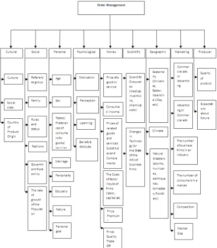
New product development, from idea creation to product introduction, requires inter-departmental communication among designers, engineers, and marketing personnel. These highlight the key areas that ought to be considered in making decisions on new product development, including customer requirements, customer satisfaction, market demand, product quality, product design, and pricing. However, no decision support system takes all of the key areas into account at the same time. Furthermore, to achieve a competitive edge in a market, sensible decisions must be made about various aspects of new product development, such as product attributes, customer segment, and promotion and marketing strategies.
In the area of Supply Chain Order Management, DSSs can be formulated through three different theoretical modeling
approaches: Available-To-Promise (ATP), Capable-To-Promise (CTP), and Profitable-To Promise
maintenance, security, safety) which represents a challenge to assign them to the cost objects.
Activity-Based Costing and Management (ABC/M) is a relatively new cost accounting and management approach that enhances the level of understanding about business operation costs; especially MOH costs. ABC/M is an accounting approach which assigns, instead of allocating, MOH costs to the activities. The importance of hybrid Supply Chain DSSs has been shown comprehensively in a recent study presented by Martinez-Olvera [9]. “As real-life business environments have become really complex, supply chains members have been forced to use hybrid business models (that is, the integration of features of two different business models).” The other three studies which have paid attention to this subject are given in [10], [11], and [12]. Martinez-Olvera [9] also discussed the optimization-based simulation models as a potential future work. In the ubiquitous environment, context awareness has played an important role in enabling the ubiquitous systems to act as intelligent decision support systems [13].
Very often, organizations lost their customers because the products are not available in warehouse when customer orders are received [14]. So, it is necessary for organizations to find the best techniques of forecasting to predict customers future orders. Simple context awareness, however, does not guarantee pro-activeness which reduces user’s required efforts by predicting the changes in relevant contexts in the future [15].Predicting users’ future context, called context prediction (CP), requires highly sophisticated inference methods capable of analyzing the given contextual data, and finding meaningful patterns from them to predict the future changes in users’ contexts. Main CP problems deal with location prediction [16] and action prediction [17]. Kaowthumrong et al. [18] use Markovian models to predict what remote control interface the user is likely to use next. Though each CP method has unique advantage over the other, they still have many pitfalls. Primary disadvantage is that most CP methods cannot provide causal relationships among target variable and related explanatory variables. If such causal relationship is extracted from target contextual data, then it can be used to do a wide variety of what-if analyses. What-if analysis allows decision makers to see possible results by changing the input conditions.
2. Bayesian Network
Bayesian belief networks (usually just called Bayesian networks) are a graphical technique used to aid reasoning and decision-making under uncertainty. Bayesian networks represent uncertainty using probabilities. Assigning a probability to an event gives an indication of how strongly we believe that the event will occur. The networks are used to compare information about a situation and make inferences. A network can provide information about the possible consequences of a situation, but can also provide information about the likely causes a key skill of effective
decision-making is the ability to correctly handle uncertainty [19].
A Bayesian belief network, usually just called a Bayesian network, is a tool that can aid decision-making under uncertainty. The network is used to analyze uncertain information and draw conclusions from the data. Although a human commander can complete a similar analysis, the network has several advantages. Once a network is constructed, it is very quick to operate. The network ensures that all of the available information is considered, as it is very easy for a human to overlook a small but vital factor. Lastly, the network can make inferences and find patterns that are sometimes too complicated for the human eye to see. Bayesian networks use probability to represent uncertainty. A probability distribution indicates the strength of our belief in uncertain information or inferences. Bayesian statistics, on the other hand, measures probabilities based only on the data observed, and use subjective probabilities where there is no data. A subjective probability is one based not on facts but on a person’s beliefs, like the odds offered by a bookmaker. A Bayesian network is a directed acyclic graph over which is defined a probability distribution. The nodes of the graph represent random variables or events. Each variable consists of a finite set of mutually exclusive states. It is possible for variables to have a continuous state, representing a numerical value such as velocity, but there are a number of limitations on their use, so we consider only variables with a finite number of states. It is usually simple to convert a continuous state to a set of finite states, so this is only a minor limitation.
The directed links between variables in the graph represent causal relationships. A link from variable A to variable B indicates that A can cause B. We say A is a parent of B, and B is a child of A. Because the network is acyclic, causal feedback is not an issue. Each variable has a probability table associated with it. Variables with no parents have a very simple probability table, giving the initial probability distribution of the variable. Variables with parents are much more complicated. These variables have conditional probability tables, which give a probability distribution for every combination of states of the variable’s parents.
There are a wide variety of Bayesian network software programs available [20]. Two of the most popular commercial programs are Hugin, from Hugin Expert A/S (www.hugin.com), and Netica, from Norsys Software Corp. (www.norsys.com). These programs provide a simple graphical user interface that can be used for both creating and running a network. To construct a Bayesian network, you must first determine the hypothesis variables. These are the variables:
• for which you are trying to determine the probability
distribution, and
• that allow you to answer your question.
events are observed, these variables allow the information to be entered into the network. Finally, intermediate, or mediating, variables are added. These variables may not be necessary, as they generally provide no extra information. However, they are useful as they allow the network structure to accurately represent the modeled system. This also dramatically reduces the size of the conditional probability tables. The network is formed by linking these variables using directed edges (arrows). It is vital to ensure that the links follow the direction specified by causality. For example, consider two variables labeled Headache and Flu. The arrow points from Flu to .Headache, because the flu causes the headache, even though it is the headache that indicates to a person that they might have the flu. Many variables need a miscellaneous state that covers anything else. This is necessary to guard against drawing the wrong conclusions from the evidence. Once the network structure is completed, the next task is to fill the probability tables.
3. Influence Diagrams
In a Bayesian network, decisions are not explicitly modeled. To allow better modeling of the decision-making process, influence diagrams have been developed. These diagrams are based on Bayesian networks, but contain two new types of nodes, decision nodes and utility nodes. Decision nodes represent a decision being made. Like a chance node (the only type of node in a Bayesian network), decision nodes have several states, usually called actions, each representing a possible outcome of the decision. Decision nodes do not have a probability table, as the node can obviously be in only one state at a time. Utility nodes are used to quantitatively represent the effects of decisions. The nodes do not have states or a probability table, nor can they have child nodes. The node contains a numerical value, or utility, for each combination of states of the parent nodes. The utility can represent any convenient numerical factor, such as cost, time or some other performance measure. The purpose of the influence diagram is to maximize (or minimize) the utility value. A Bayesian network can generally be extended into an influence diagram. Decision nodes are added wherever a decision must be made. The parents of a decision node are the variables that will affect the outcome of the decision being made and the children are the variables affected by the decision. For an influence diagram to be valid, there must be a directed path through each of the decision variables, so that the decisions can be made in sequence. The utility nodes are entered wherever the value of the utility can be measured, and are usually at the very bottom of the network so that all factors can be taken into account. Several Bayesian network software programs can solve influence diagrams. The diagrams are compiled as an ordinary network would be, evidence is entered and the probabilities are propagated. The software gives each action of a decision node a numerical utility value. As each decision is encountered, the best choice is the action with the highest
or lowest utility (depending on whether you wish to maximize or minimize the utility value).As more decisions are made and more evidence is entered, the utilities of the remaining decision nodes are updated. To work correctly an influence diagram requires an effective numerical utility, which is usually cost. Another decision-making tool related to the influence diagram is the decision tree. Unlike Bayesian networks and influence diagrams, the decision tree has a strict tree structure. Each chance node or decision node has one child for each of its states or actions and each branch of the tree ends in a utility node. Each decision has two actions, and each chance node has three possible outcomes. The utility nodes give the utility of each possible course of action. Influence diagrams can often be converted into decision trees. The decision tree is much larger than its corresponding influence diagram, because there must be one leaf for each possible decision sequence, and is correspondingly harder to construct. The tree has the advantage of presenting the full decision-making process to the user, but despite this an influence diagram is usually a better choice than a decision tree. Because an influence tree must provide a directed path through all decision nodes, there are some situations that the diagrams cannot model. These include situations where the decisions to be made, or their sequence, changes depending on the result of an earlier decision. It is in these situations that a decision tree is most useful. Most Bayesian network software is incapable of running decision trees. However there are commercial software packages that can provide this capability. Some are stand-alone products and several are add-ins for the Microsoft Excel spreadsheet program. They usually work in a similar way to the Bayesian network software. When all of the information is entered, the utilities are propagated up the tree to the root. As each decision is reached, the best choice is the one with the highest (or lowest) utility value. As with the influence diagrams, decision trees require a consistent utility measurement, and so the same difficulties apply in determining a suitable utility. Generally a decision tree is only useful to directly model a decision-making process. Any other systems should be modeled using an influence diagram wherever possible.
4. New Product Development Order
Management System
the parameters being employed in the prediction of customers’ orders for a new product being developed in NPD process. The drawback of complicated decision support problems are the complexities involved in interpreting causal relationships among decision variables. Therefore, Bayesian Network (BN) has shown excellent decision support competence due to its flexible structure allowing itself to extract appropriate and robust causal relationships among target variable and related explanatory variables. We make use of a decision support BN as a prediction aid for order management in a new product development process. All predictions are based on past data. Due to past data we
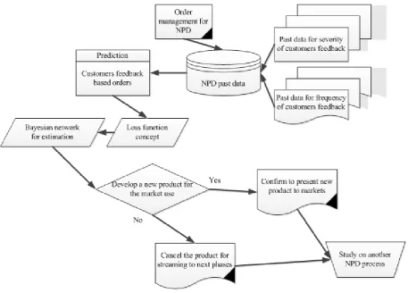
[image:4.595.86.526.229.731.2]employ two properties of frequency and severity of an occurrence effective on orders to model the decision system. Thus, we develop a loss function for the proposed influence diagram and compute the loss using a Bayesian network to determine the NPD minimum loss incurred with respect to customer order prediction for the newly product before its entrance to the market. This helps the managers to prevent a big loss of income for NPD process since they can predict customers’ behavior against the new product before the phase of manufacturing (in which added specifications are included). A configuration of the proposed DSS in order management for NPD process is depicted in Figure 2.
Figure 2. A DSS for NPD order management
5. Loss Function Estimation for Order
Management
The model applied in the present work belongs to the applied measurement approach (AMA) and it is called the loss distribution approach (LDA). It is characterized by the categorization of the losses in terms of ‘Frequency’ (the number of loss events during a certain time period) and ‘Severity’ (the impact of the event in terms of economic loss). Formally, for each intersection r (where r = 1, . . . , R) and for a given time period t, the total operational loss could be defined as the sum of a random number nt of losses:
Lrt= Xr1+ Xr2+· · ·+Xr
n
t, (1) where Lrt denotes the total operational loss, Xr1, . . . , Xrn
tdenote individual loss severities and nt denotes the frequency,
for t =1, . . . , T, T representing the number of time periods. Note that, for each intersection and for each time period, the total loss can be expressed as
Lt= st· nt, (2)
where nt is the frequency, defined as before, and
st(commonly referred to as the severity) is the mean loss for
that period. The LDA assumes that, for each time period: (1) the individual losses {Xrq}, where q = 1, . . . , nt, are
independent and identically distributed random variables;
(2) the distribution of the frequency nt is independent of
the distribution of the severities {Xrq}, for q = 1,… , nt. This
implies that nt is independent of st;
(3) besides, Lrt, for t = 1, . . . ,T, are independent and
identically distributed random variables.
For a given intersection, we construct a discrete probability density of the number of loss events nt during the
considered time period and nt continuous probability
densities of the loss severities. Now, if we express the likelihood function for each intersection in a general way, we obtain the following equation.
Indicating the severity distribution with
f
( )
x
qξ
and the frequency distribution withf
( )
n
tψ
, whereξ
denotes the parameter vector of the severity distribution andψ
denotes the parameter vector of the frequency distribution, we obtain the following form:(
)
1 1
x,n ,
T nt(
q(
t)
t q
L
ψ ξ
f x
ξ
f n
ψ
= =
=
∏ ∏
. (3)Exponential, the Gamma and the Pareto distributions. For more details about these distributions see [21].
Our first problem is to estimate, on the basis of data, the parameters of the frequency and severity distributions, denoted by
ψ
andξ
, respectively, in equation (3). The classical approach suggests the employment of the method of moments or the method of maximum likelihood, as described, for example, by Gourieroux and Monfort [22]. An alternative approach is the Bayesian method, which allows the combination of quantitative data, coming from the time series of operational losses, and prior information, represented by expert opinions. In this paper we estimate the parameters with the maximum likelihood method and with the Bayesian method, making some comparisons between the classical and the Bayesian approaches. In particular, we choose the maximum likelihood method because of its good asymptotic properties, since the MLE converges almost surely to the true value of the parameter, under fairly general conditions. Once the parameters have been estimated, the marginals are defined and the operational loss distribution has to be identified.6. Bayesian Approach
Suppose a continuous probability distribution with probability density function (pdf) ƒΘ is assigned to an
uncertain quantity Θ. In the conventional language of mathematical probability theory Θ would be a "random variable" [23]. The probability that the event B will be the outcome of an experiment depends on Θ; it is P(B | Θ). As a function of Θ this is the likelihood function:
(
θ
)
θ
=
P
B
Θ
=
L
(
)
(4)Then the posterior probability distribution of Θ, i.e. the conditional probability distribution of Θ given the observed data B, has probability density function
( )
θ
B
f
θ
L
( )
B
θ
f
Θ=
constant.
Θ(
)
, (5)where the "constant" is a normalizing constant so chosen as to make the integral of the function equal to 1, so that it is indeed a probability density function. This is the form of Bayes' theorem actually considered by Thomas Bayes [24]. In other words, Bayes' theorem says:
To get the posterior probability distribution, multiply the prior probability distribution by the likelihood function and then normalize.
More generally still, the new data B may be the value of an observed continuously distributed random variable X. The probability that it has any particular value is therefore 0. In such a case, the likelihood function is the value of a probability density function of X given Θ, rather than a probability of B given Θ:
(
θ
)
θ
=
f
x
Θ
=
L
(
)
X . (6)Bayes's rule provides the framework for combining prior information with sample data. In this reference, we apply Bayes's rule for combining prior information on the assumed distribution's parameter(s) θ with sample data in order to make inferences based on the model. The prior knowledge about the parameter(s) is expressed in terms of a pdf f(θ), called the prior distribution. The posterior distribution of θ
given the sample data, using Bayes rule, provides the updated information about the parameters θ. This is expressed with the following posterior pdf:
(
)
(
(
)
)
( )
( )
∫
=
ε
θ
θ
ϕ
θ
θ
ϕ
θ
θ
d
L
L
f
Data
Data
Data
. (7)where,
θ is a vector of the parameters of the chosen distribution,
ε
is the range of θ,L(Data|θ) is the likelihood function based on the chosen distribution and data,
f(θ) is the prior distribution for each of the parameters. The integral in equation (7) is often referred to as the marginal probability and can be interpreted as the probability of obtaining the sample data given a prior distribution and it's a constant number. Generally, the integral in equation (7) does not have a closed form solution and numerical methods are needed for its solution.
As can be seen from equation (7), there is a significant difference between classical and Bayesian statistics. First, the idea of prior information does not exist in classical statistics. All inferences in classical statistics are based on the sample data. On the other hand, in the Bayesian framework, prior information constitutes the basis of the theory. Another difference is in the overall approach of making inferences and their interpretation. For example, in Bayesian analysis the parameters of the distribution to be "fitted" are the random variables. In reality, there is no distribution fitted to the data in the Bayesian case.
For instance, consider the case where data is obtained from a reliability test. Based on prior experience on a similar product, the analyst believes that shape parameter of the Weibull distribution has a value between β1 and β2 and wants to utilize this information. This can be achieved by using the Bayes theorem. At this point, the analyst is automatically forcing the Weibull distribution as a model for the data and with a shape parameter between β1 and β2. In this example, the range of values for the shape parameter is the prior distribution, which in this case is Uniform. By applying equation (7), the posterior distribution of the shape parameter will be obtained. Thus, we end up with a distribution for the parameter rather than an estimate of the parameter, as in classical statistics.
for that parameter is then obtained using equation (7). This posterior distribution of the parameter may or may not resemble in form the assumed prior distribution. In other words, in this example the prior distribution of β was assumed to be uniform but the posterior is most likely not a uniform distribution.
The question now becomes: what is the value of the shape parameter? What about the reliability and other results of interest? In order to answer these questions, we have to remember that in the Bayesian framework all of these metrics are random variables. Therefore, in order to obtain an estimate, a probability needs to be specified or we can use the expected value of the posterior distribution.
In order to demonstrate the procedure of obtaining results from the posterior distribution, we will rewrite equation (7) for a single parameter θ1:
(
)
(
)
( )
(
) ( )
∫
=
εθ
θ
ϕ
θ
θ
ϕ
θ
θ
1 1 1 1 1 1Data
Data
Data
d
L
L
f
. (8)The expected value (or mean value) of the parameter θ1 can be obtained as follows:
(
)
∫
=
εθ
θ
θ
θ
1)
1.
1Data
1(
f
d
E
. (9)7. Numerical Study
Here, we work out an application of the proposed methodology for NPD order management. As stated, an influence diagram is effective to determine order for a new product which should have less operational loss. The data set we use in our analysis contains the operational losses of an NPD process considering the influence diagram in a time period. For a total of 12 monthly observations,27 loss events, distributed over six intersections exist. From intersection we mean each pair of multiplied severity and frequency. The aim is to conceptualize the loss associated with influence diagram data.
Now, we examine all the combinations of frequency and severity and, for each of them, we will apply the Bayesian approach to estimate the parameters.
Let us consider the Poisson–Exponential combination. For each intersection we have, for t = 1,..., M:
( )
t
n
Poisson
λ
and
1
,...,
nt( )
X
X
Exponential
θ
The likelihood function is therefore, substituting in equation (3) the Poisson distribution for
f n
( )
tθ
and the Exponential distribution forf x
( )
jη
:(
)
1 1
exp( )
x,n ,
exp(
)
.
!
t t
n n
M
j
t j t
L
x
n
λ λ
λ θ
θ
θ
= =
−
=
−
∏ ∏
We choose independent conjugate priors for the parameters
λ
andθ
, in order to obtain a posterior belonging to the same class of distributions as the prior. Therefore we set( , )
a b
λ
Γ
and
( , )
c d
θ
Γ
.According to Bayes’ Theorem, the conditional posterior of the
λ
parameter is computed by multiplying the likelihood function by the prior distribution. The form we get is a Gamma, as specified in the following:(
)
1
x,n,
M t;
t
n a M b
π λ
θ
=
Γ
+
+
∑
.Also, the conditional posterior distribution for
θ
is a standard form,(
)
1 1 1
x,n,
M t;
M nt jt
n c
t jx d
π θ
λ
= = =
Γ
+
+
∑
∑∑
.Table 1 lists all the posteriors computed for the combination Poisson/Exponential from intersection 1 to intersection 6.
Using the values given in Table 1, the operational losses are obtained. The operational losses are the decision factors in NPD decisions. Due to operational losses obtained as a prediction from the order management system NPD decision is impacted. One can set a threshold for the loss values and accept/reject with respect to that threshold. Then the values below the threshold implies that the analysis predict that if the management invest on the NPD process, more benefit (less loss) will be obtained.
Table 1. Posteriors computed for the combination Poisson/Exponential Poisson/Exponential priors
λ
θ
A b c d
Intersection 1 19.6 13 4.2 9.3 Intersection 2 23.4 9 3.8 8.5 Intersection 3 17.1 12 5.1 11 Intersection 4 25.3 14.3 6.9 10.4 Intersection 5 14.1 6.5 8.2 13 Intersection 6 27.8 18.4 7.5 11
The advantages of the proposed methodology are:
● Bold role of research and development (R&D) center in NPD process
● Predicting the profit before investment on NPD process
● Controlling uncertainty and dynamism of future analysis for NPD
distributions
● Usefulness of the collected data (past data) for future analysis of NPD
● Maximizing the expected benefit form an NPD process
● Competitive advantage of the management equipped with the proposed methodology
● Reducing the risk exist in the NPD process
● Close relationship between order management and NPD process
To sum up, the proposed methodology with the above capabilities is a significant tool for the NPD process since the current market is very competitive and absorbing large amount of markets requires subtle analysis and decision making.
8. Conclusions
Here, we proposed a new product development (NPD) order management decision support system considering past data of a proposed influence diagram aiming to find the ones with more convergence for value added purposes. The influence diagram fields were related to customers’ order. A loss function was considered to model the influence diagram. Due to stochastic and dynamic nature of data in NPD process, Bayesian approach was employed to estimate the loss function. The applicability and effectiveness of the approach was presented in a numerical study. The advantages of the proposed methodology were illustrated.
REFERENCES
[1] X. Gao, Z. Li, L. Li, A processmodel for concurrent design in manufacturing enterprise information systems, Enterprise Information Systems 2 (1) (2008) 33–46.
[2] S.L. Chan , W.H. Ip, A dynamic decision support system to predict the value of customer for new product development , Decision Support Systems 52 (2011) 178–188.
[3] G. Alexouda, A user-friendly marketing decision support system for the product line design using evolutionary algorithms, Decision Support Systems 38 (2005) 495–509. [4] J.A. Harding, K. Popplewell, R.Y.K. Fung, A.R. Omar, An
intelligent information framework relating customer requirements and product characteristics, Computers in Industry 44 (2001) 51–65.
[5] A. Herrmann, F. Huber, C. Braunstein, Market-driven product and service design: Bridging the gap between customer needs, quality management, and customersatisfaction, International Journal of Production Economics 66 (2000) 77–96.
[6] L.P. Khoo, C.H. Chen, W. Yan, An investigation on a prototype customer-oriented information system for product concept development, Computers in Industry 49(2002) 157–174.
[7] L. Xu, Z. Li, S. Li, F. Tang, A decision support system for product design in concurrent engineering, Decision Support
Systems 47 (2007) 2029–2042.
[8] Amir H. Khataie a, Akif A. Bulgak a, Juan J. Segovia ,2011, Activity-Based Costing and Management applied in a hybrid Decision Support System for order management, Decision Support Systems 52 (2011) 142–156.
[9] C. Martinez-Olvera, Benefits of using hybrid business models within a supply chain, International Journal of Production Economics 120 (2009) 501–511.
[10] D. Li, C. O'Brien, Integrated decision modeling of supply chain efficiency, International Journal of Production Economics 59 (1999) 147–157.
[11] D. Li, C. O'Brien, A quantitative analysis of relationships between product types and supply chain strategies, International Journal of Production Economics 73 (2001) 29–39.
[12] W. Sen, S. Pokharel, W.Y. Lei, Supply chain positioning strategy integration, evaluation, simulation, and optimization, Computers and Industrial Engineering 46 (2004) 781–792. [13] Cook, D. J., Augusto, J. C., & Jakkula, V. R. (2009).
Ambient intelligence: Technologies, applications, and opportunities. Pervasive and Mobile Computing, 5, 277–298. [14] Malihe Manzouri, Mohd Nizam Ab Rahman and Haslina
Arshad, Order Management in Supply Chain: A Case Study in Automotive Companies, American J. of Engineering and Applied Sciences 4 (3): 372-379, 2011.
[15] Mayrhofer, R., Radi, H., & Ferscha, A. (2003). Recognizing and predicting context by learning from user behavior. International conference on advances in Mobile Multimedia (MoMM) (Vol. 171). Austrian Computer Society (OCG). [16] Petzold, J., Bagci, F., Trumler, W., & Ungerer, T. (2005).
Next location prediction within a smart office building. Cognitive Science, 577, 69 [Research Paper, University of Sussex CSRP].
[17] Kim, E., Helal, S., & Cook, D. (2010). Human activity recognition and pattern discovery. IEEE Pervasive Computing, 9, 48–53.
[18] Kaowthumrong, K., Lebsack, J., Han, R. (2002). Automated selection of the active device in interactive multi-device smart spaces. In Workshop at UbiComp 2002: Supporting spontaneous interaction in ubiquitous computing settings. [19] U.S. Navy, 1995, .Naval Doctrine Publication 6: Command
and Control - Chapter 2: The Process of Command and Control.
[20] Murphy, K. P. 2002, .Software Packages for Graphical Models / Bayesian Networks.,<http://www.cs.berkeley.edu/ ~murphyk/Bayes/bnsoft.html>, 8 January 2004
[21] Johnson, N.L., Kotz, S. and Balakrishnan, N. (1994). Continuous Univariate Distributions, vol. 1, second ed.Wiley, NewYork.
[22] Gourieroux, C. and Monfort, A. (1995). Statistics and Econometric Models. Cambridge University Press, Cambridge.
[23] Lehmann, E. L.; Casella, G. (1998). Theory of Point Estimation. Springer. p. 2nd ed. ISBN 0-387-98502-6. [24] Berger, J.O. (1985). Statistical decision theory and Bayesian