A More Accurate and Straightforward Method for Evaluating Singular Integrals

(1)

A More Accurate and Straightforward Method for

Evaluating Singular Integrals

M. Kamrul Hasan

1,*

_{, M. Ashraful Huq}

1

_{, M. Habibur Rahaman}

1

_{, B.M. Ikramul Haque}

1,2

1_{Department of Mathematics, Rajshahi University of Engineering and Technology, Bangladesh} 2_{Department of Mathematics, Khulna University of Engineering and Technology, Bangladesh}

Abstract

Recently, a straightforward formula has been presented for evaluating singular integrals. Earlier extrapolation technique was used to guess the functional values at the singular points since most of the classical formulae contain both ends points. In this article a more accurate straightforward formula is presented for evaluating singular integrals. The new formula converges faster than others existing formulae. The Romberg integration scheme of this method also converges faster.

Keywords

Numerical Integral, Singular Integral, Newton-Cotes Formulae, Romberg Integration Scheme

1. Introduction

The closed form Newton-Cotes formulae [1] such as Trapezoidal rule, Simpson rules are widely used for evaluating definite integrals. But these formulae are not used directly for evaluating integrals when singularities arise. Earlier Fox [2] used classical (numerical) formulae for evaluating singular integrals. However, most the classical formulae (also their composite forms) contain ends points. For the singular integrals, the functional values of the ends (sometimes one end point) are indefinite. For this reason Fox [2] used extrapolation technique to evaluate the functional values at the singular points. Delves [3] evaluated the principal value of singular integrals by Newton’s-Cote and modified Gaussian methods. Latter Hunter [4] evaluated the principal value of singular integrals by modified Trapezoidal rule. Latter than several author’s [5]-[9] evaluated singular integrals by Gauss quadrature, modified/extended Gauss quadrature methods. The derivation as well as utilization of these methods is laborious.

Recently, Huq et al [10] has developed a simple and straightforward formula for evaluating singular integrals,

∫

=

b

a

y

x

dx

I

(

)

(1)

where

y

(

x

)

is singular at

x

=

a

or/and

x

=

b

. The formula excludes the end points and used directly for the singular integrals.

In general the composite classical formulae are used by equally sub-divided an interval

[

a

,

b

]

. But it can be show that the result is improved if we properly select sub-divisions of the interval. To verify this statement, let us rewrite integral Eq. (1) as

∫

+

= b

a

dx x y dx x y I

x x

x

) ( ) ( )

( (2)

where

a

<

x

<

b

. According to Trapezoidal rule, it has an approximate value

2 / ))) ( ) ( )( ( )) ( ) ( )( (( )

( a y a y b y y b

I x = x− + x + −x x + (3)

Clearly

I

(

x

)

has a nearest value to the exact result,

I

, if

I

′

(

x

)

=

0

. Differentiating Eq. (3) with respect to

x

and simplifying, we obtain

a

b

a

y

b

y

−

=

′

₍

x

₎

(

)

(

)

(4)

Thus

x

satisfy Eq. (4) (well known as Mean Value Theorem). In a similar way, if the interval is subdivided into

2 ≥

n

parts,

I

becomes a function of

x

_i ,

1 ,

,

2 ,

1 −

=

n

i



and applying

∂

I

/

∂

x

_i

=

0

, we obtain from the following set of equations

2 2 1

)

(

)

(

)

(

− −

−

=

₋

−

′

i i

i

y

x

_x

x

(5)

where

x

₀

=

a

and

x

_n

=

b

. From Eq. (5), we see that

=

−

=

b

a

n

i

(

)

/

(2)

when

y

=

x

2 . Otherwise, the values of

x

_i ,

1 ,

,

2 ,

1 −

=

n

i



are different. When

y

=

x

,

a

=

0

and

b

=

1

, we obtain

x

_i

=

i

2

/

n

2 . If

n

=

2

,

4 /

1

=

x

. But the middle point of this interval is

1 /

2

, which is much larger than

x

₁

.

In this case, we obtain

625 .

0 )

4 /

1 (

=

I

and

I

(

1 /

2 )

≈

0 .

6036

. The exact value

I

is

2 /

3

. Thus

I

(

1 /

4 )

is closer to the exact result. When

n

=

10

, we obtain

x

₁

=

1 /

100

,

100 /

4

2

=



x

₉

=

81 /

100

. In this case we

calculated

I

(

1 /

100 ,

4 /

100 ,



,

81 /

100 )

=

0 .

665

. For the classical composite formula,

10 /

9 ...,

,

10 /

2 ,

10 /

1

₂ ₉

1

=

x

=

x

=

x

and we obtain

660509

.

0 )

10 /

9 ,

,

10 /

2 ,

10 /

1 (



=

I

. This investigation

indicates that proper choice of sub-divisions of an interval is important. It is noted that the classical composite formulae (Trapezoidal, Simpson's etc.) may be used when

2 1 2 3 1

2

−

x

,

x

−

x

,

x

n−

−

x

n−

x

are almost same. In [10],

a second order formula has been developed by choosing unequal sub-divisions of an interval as

h

x

h

x

₀

,

₀

+

,

₀

+

3

. The main benefit of the new method is that it excludes the functional value at

x

₀. On the contrary, Simpson's 1₃ formula was derived by choosing

h

x

h

x

₀

,

₀

+

,

₀

+

2

. In [10], it has been shown that the new formula measures better result than Simpson's 1₃ formula for many functions especially having a singular point. In this article a more accurate third order formula is presented for evaluating such singular integrals by considering unequal sub-divisions of an interval which again excludes the functional value at

x

₀. The composite of all higher order formulae give better result when the interval is divided unequally; but the nearest result can be found by applying

∂

I

/

∂

x

_i

=

0

. It is difficult to solve the similar equations to Eq. (5) for any higher order formula rather than Trapezoidal. Fortunately the result is very close the nearest result when

x

_i,

i

=

1 ,

2 ,



,

n

−

1

are determined from Eq. (5). The aim of this article is to derive a more accurate formula for evaluating singular integrals.

2. Derivation of the Present Formula

An interpolation formula is usually utilized for determination of a numerical integration formula such as Trapezoidal, Simpson’s 1₃ _{and Simpson’s}

8

3 _{etc. All} these formula are established by Newton's forward formula. Recently, Huq et al [10] has used Lagrange’s formula to drive an integration formula, e.g

1 3 3 0

3 ₃

( ) [3 ], ( ) / 3

4 0

x

h

y x dx= y +y h= x x−

∫

(6)

considering three points

x

₀

,

x

₁

,

x

₃ together with

h

x

₁

=

₀

+

and

x

₃

=

x

₁

+

2 h

(details in [10]). It is clear that formula (6) excludes

y

₀ and thus it is used directly if

y

(

x

)

is singular point at

x

₀.

On the contrary, another formula

0 2 3 0

3 ₃

( ) [ 3 ], ( ) / 3

4 0

x

h

y x dx= y + y h= x −x

∫

₍₇₎

was derived [10] by considering three points

x

₀

,

x

₂

,

x

₃ together with

x

₂

=

x

₀

+

2 h

and

x

₃

=

x

₀

+

3 h

, which is used directly when

y

(

x

)

is singular point at

x

₃. Huq et al [10] also derived another formula which covers both singularities (i.e., for

x

=

a

and

x

=

b

) as

1 3 5 6 0

6 ₃

( ) [3 2 3 ], ( ) / 6

4 0

x

h

y x dx= y+ y + y h= x −x

∫

(8)

A general form of formula (8) in the interval

[

a

,

b

]

was derived [10] as

...)]

(

3 ...)

(

2 ...)

(

3 [

4

3 )

(

17 11 5 15

9 3

13 7 1

+

=

∫

y

h

dx

x

y

b

a (9)

where,

h

=

(

b

−

a

)

/

6 n

,

n

=

1 ,

2 ,

3 ,...

The formula (9) also excludes

y

₀ and

y

_n, it is useful directly when

y

(

x

)

is singular at

a

or/and

b

.

In order to derive a more accurate new formula, we have considered four points

x

₀

,

x

₁

,

x

₄

,

x

₆ together with

x

₁

=

x

₀

+

h

,

x

₄

=

x

₀

+

4 h

and

x

₆

=

x

₀

+

6 h

(i.e.,

x

₂

,

x

₃

,

x

₅ has been ignored) and integrating from

0

x

to

x

₆ , gives the form as (see Appendix)

6 0

( ) / 6

6 ₃

( ) ₅[4 ₁ 5 ₄ ₆],

0 h x x

x _h

y x dx y y y

x∫ = + + = − (10)

y

₀ and it is useful directly when

y

(

x

)

is singular at

x

₀. On the contrary, another formula has been obtained as (see Appendix)

0 2 5 ( 6 0) / 6

6 ₃

( ) ₅[ 5 4 ],

0 h x x

x _h

y x dx y y y

x∫ = + + = − (11)

by considered four points

x

₀

,

x

₂

,

x

₅

,

x

₆ together withx₂=x₀+2h,

x

₅

=

x

₀

+

5 h

and x6 =x0+6h. The formula (11) also excludes

y

₆and it is useful directly when

)

(

x

(3)

formula like as (11) with four points

x

₆

=

x

₀

+

6 h

,

h

x

₈

=

₀

+

8

,

x

₁₁

=

x

₀

+

11 h

,

x

₁₂

=

x

₀

+

12 h

, has been obtained

₆ ₈ ₁₁ ₁₂ ₆ 12

( ) / 6 6

3

( ) ₅[ 5 4 ], h x x

x _h

y x dx y y y

x∫ = + + = − (12)

Now a new formula which covers both singularities (i.e., for

x

=

a

and

x

=

b

) has been obtained by combining formulae of (10) and (12) as

] 4 8 5 6 2 5 4 [ 5 3 )

( 1 4 11

12

0

y y y y y h x

x∫y x dx= + + + +

,

12 /

)

(

x

₁₂

x

₀

h

=

−

(13)

In general the formula (13) can be written a

..)] 23 (

4 ..) 20 8 ( 5 ..) 18 6 ( 2

..) 16 (

5 ..) 13 ( 4 [ 5 3 ) (

11 4 1

+ + + + + + + + +

+ + + + + + =

∫

y y y

y y

y

y y y

y h dx x y

b

a

(14) where,

h

=

(

b

−

a

)

/

12 n

,

n

=

1 ,

2 ,

3 ,...

.

y

₀ and

y

_n, it is useful directly when

y

(

x

)

is singular at

a

or/and

b

.

3. Error of the Present Formula

Tailor’s series is usually used for evaluating the order of error [1]. The error of the new formulae (14) has been calculated as

.

,

20 )

(

)

(

b

−

a

h

4

y

iv

x

_a

_<

_x

_<

_b

(15)

4. Examples

4.1. Let us consider a lower singular integral

dx

x

I

=

1

_∫

0

1

(16)

Obviously

0

is the singular point of integral (16). The formula (14) with

h

=

1 /

12

,

h

=

1 /

24

and

h

=

1 /

48

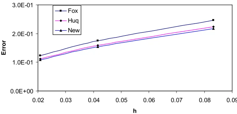
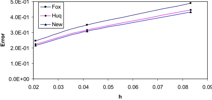
the approximate results of integral (16) have been obtained 1.7823337861518145, 1.8460831095334458 and 1.8911641218387858 respectively. The exact value of this integral is 2. Comparison the errors of this integral obtained by Fox [2], Huq et al [10] and the new methods are shown in Fig.1. Romberg integration scheme of the results of integral (16) by Fox [2], Huq et al [10] and the new method has been given in Tables 4.1(a), 4.1(b) and 4.1(c) respectively.

0.0E+00 1.0E-01 2.0E-01 3.0E-01

0.02 0.03 0.04 0.05 0.06 0.07 0.08 0.09 h

Erro

r

[image:3.595.114.494.435.618.2]

Fox Huq New

Figure 1. Comparison the errors of the integral (16) obtained by three methods.

Table 4.1(a). Approximate value of the integral (16) presented by Fox [2]

7190366 1.99999904

) , , ( 1146543 1.99977445

) , (

30150734 1.99910066

) , (

35780040 1.87656174

) (

90464053 1.82552536

) (

8191686 1.75362812

) (

481 241 121 481

241 241 121

481 241 121

= =

=

= = =

U U

U

(4)

Table 4.1(b). Approximate value of the integral (16) presented by Huq et al [10] formula (9)

05534177 1.99999983

) , , ( 71029545 1.99999788

) , (

53459954 1.99996873

) , (

63083991 1.88782433

) (

02297469 1.84136053

) (

05669431 1.77566286

) (

481 241 121 481

241 241 121

481 241 121

= =

=

= = =

H H

H

H H H

Table 4.1(c). Approximate value of the integral (16) obtained by the new formula (14)

46530703

2.00000009

)

,

(

31518463

1.99999931

)

,

(

06334879

1.99998759

)

,

(

18387858

1.89116412

)

(

95334458

1.84608310

)

(

61518145

1.78233378

)

(

481 241 121 481

241 241 121

481 241 121

=

N

4.2. Let us Consider a Another Lower Singular Integral

∫

− = 1

0xlnxdx

I (17)

Choosing

h

=

1 /

12

,

h

=

1 /

24

and

h

=

1 /

48

_{, formula (14) has been utilized and measured values}

77129326

0.25115309

,

0.25028879

28867005

and

0.25007222

79339513

_{respectively. The exact value of this}

integral is

0 .

25 .

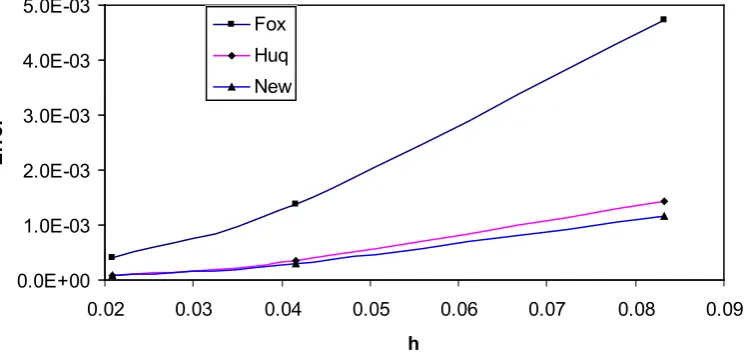
Comparison the errors of this integral obtained by Fox [2], Huq et al [10] and the new methods are shown in Fig.2. Romberg integration scheme of the results of integral (17) by these methods have been given in Tables 4.2(a), 4.2(b) and 4.2(c) respectively.

0.0E+00 1.0E-03 2.0E-03 3.0E-03 4.0E-03 5.0E-03

0.02 0.03 0.04 0.05 0.06 0.07 0.08 0.09 h

Erro

r

[image:4.595.123.496.437.613.2]

Fox Huq New

816844634 0.25000005

) , , ( 011446614 0.24980376

) , (

189179819 0.24937514

) , (

9428990 0.25039568

) (

82865298 0.25138223

) (

89444158 0.25472739

) (

481 241 121 481

241 241 121

481 241 121

= =

=

= = =

U U

U

(5)

50078764 0.25000000

) , , ( 011340055 0.25000013

) , (

66962632 0.25000200

) , (

24202118 0.25008937

) (

93406455 0.25035709

) (

72737922 0.25142237

) (

481 241 121 481

241 241 121

481 241 121

= =

=

= = =

H H

H

H H H

617226232 0.24999999

) , , ( 96163682 0.25000003

) , (

127795643 0.25000069

) , (

79339513 0.25007222

) (

28867005 0.25028879

) (

77129326 0.25115309

) (

481 241 121 481

241 241 121

481 241 121

= =

=

= = =

N N

N

N N N

4.3. Let us Consider a Stronger Lower Singular Integral

dx

x

e

I

=

1

_∫

−x

0 43

(18)

Choosing

h

=

1 /

12

,

h

=

1 /

24

and

h

=

1 /

48

_{, formula (14) has been utilized and measured values}

90762165

1.95605738

,

2.18385049

97275354

and

2.37461693

62833469

_{respectively. The exact value of}

this integral is

3.37935437

9028409

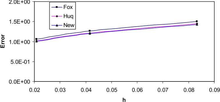
. Comparison the errors of this integral obtained by Fox [2], Huq et al [10] and the new methods are shown in Fig.3. Romberg integration scheme of the results of integral (18) by these methods have been given in Tables 4.3(a), 4.3(b) and 4.3(c) respectively.

0.0E+00 5.0E-01 1.0E+00 1.5E+00 2.0E+00

0.02 0.03 0.04 0.05 0.06 0.07 0.08 0.09 h

Er

ro

r

[image:5.595.118.492.436.610.2]

Fox Huq New

38112667 3.38266536

) , , ( 9608616 3.38448551

) , (

70006754 3.38994598

) , (

60719088 2.31841702

) (

20145315 2.11670928

) (

83485327 1.87580383

) (

481 241 121 481

241 241 121

481 241 121

= =

=

= = =

U U

U

(6)

54989197

3.38287034

)

,

(

1583055

3.38323157

)

,

(

2845063

3.38864996

)

,

(

83880760

2.36059033

)

(

09724293

2.16709934

)

(

19781286

1.93597327

)

(

481 241 121 481

241 241 121

481 241 121

=

H

7517159 3.38252978

) , , ( 36188748 3.38285828

) , (

5144628 3.38778572

) , (

62833469 2.37461693

) (

97275354 2.18385049

) (

90762165 1.95605738

) (

481 241 121 481

241 241 121

481 241 121

= =

=

= = =

N N

N

N N N

4.4. Let us Consider an Upper Singular Integral

dx x e

I

_∫

x

− =1 −

0 (1 2)

(19)

Obviously

1

is the singular point of integral (19). Choosing

h

=

1 /

12

,

h

=

1 /

24

and

h

=

1 /

48

_{, formula (14) has} been utilized and measured values

0.79448520

79547432

,

0.81698226

43136603

and

0.83322797

89351417

respectively. The exact value of this integral is

0.87308424

26508668

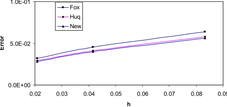
. Comparison the errors of this integral among these methods are shown in Fig.4. Romberg integration scheme of the results of integral (19) by these methods have been given in Tables 4.4(a), 4.4(b) and 4.4(c) respectively.

0.0E+00 5.0E-02 1.0E-01

0.02 0.03 0.04 0.05 0.06 0.07 0.08 0.09 h

Er

ro

r

Fox Huq New

43255449

0.87286830

)

,

(

9367418

0.87294753

)

,

(

44930386

0.87318524

)

,

(

37861391

0.84106217

)

(

29211492

0.82785482

)

(

75179827

0.80907834

)

(

481 241 121 481

241 241 121

481 241 121

=

U

[image:6.595.118.493.448.626.2]

(7)

05937489

0.87285160

)

,

(

75921011

0.87282482

)

,

(

25673849

0.87242323

)

,

(

21348564

0.84398290

)

(

54455118

0.83203618

)

(

27834307

0.81530732

)

(

481 241 121 481

241 241 121

481 241 121

=

H

60233444

0.87287877

)

,

(

38520584

0.87285317

)

,

(

12827638

0.87246914

)

,

(

59691604

0.84484218

)

(

48925955

0.83323965

)

(

95848572

0.81699026

)

(

481 241 121 481

241 241 121

481 241 121

=

N

4.5. Let us Consider a Both Singular Integral

dx

x

I

_∫

−

=

1

0

(

1 )

1

₍₂₀₎

Obviously

0

and1 are singular points of integral (20). Choosing

h

=

1 /

12

,

h

=

1 /

24

and

h

=

1 /

48

_{, formula (14)} has been utilized and measured values

2.65196914

10133683

,

2.79384301

68849990

and

61839047

2.89516599

respectively. The exact value of this integral is

3.14159265

3589793

. Comparison the errors of this integral among these methods are shown in Fig.5. Romberg integration scheme of the results of integral (20) by these methods have been given in Tables 4.5(a), 4.5(b) and 4.5(c) respectively.

0.0E+00 1.0E-01 2.0E-01 3.0E-01 4.0E-01 5.0E-01

0.02 0.03 0.04 0.05 0.06 0.07 0.08 0.09 h

Er

ro

r

[image:7.595.121.490.451.625.2]

Fox Huq New

Table 4.5(a). Approximate value of the integral (20) presented Fox [2]

1929586

3.14092279

)

1 ,

1 (

69873712

3.13978130

)

1 ,

24

1 (

21607266

3.13635685

)

24

1 ,

1 (

238584

8575718811

.

1 )

1 (

66749424

1.78768452

)

1 (

4573801

.689014923

1 )

1 (

48 24 12 48

12

48 24 12

=

U

(8)

920859

3.14087764

)

1 ,

1 (

696028

3.14078067

)

1 ,

1 (

32356237

3.13932609

)

1 ,

1 (

88495735

2.91748415

)

1 (

26174293

2.82499171

)

1 (

90452266

2.69479014

)

1 (

48 24 12 48 24 24 12 48 24 12

=

H

_1499516 3.14096289 ) 1 , 1 , 1 ( 78184646 3.14087847 ) 1 , 1 ( 26026885 3.13961227 ) 1 , 1 ( 20992149 2.92413431 ) 1 ( 90930597 2.83435593 ) 1 ( 57530864 2.70791462 ) 1 ( 48 24 12 48 24 24 12 48 24 12 = = = = = = N N N N N N

5. Results and Discussions

A more accurate and straightforward formula has been developed for evaluating singular integrals. It has been mentioned that Huq et al [10] is a straightforward method for evaluating singular integrals. Moreover, Huq et al [10] gives more accurate results than Fox [2] method. The new method gives more accurate results than Huq et al [10] as well as Fox [2] (see Fig.1-Fig. 5).

Seeing Tables 4.1(a)-4.5(c), it is clear that the new method converges faster than Fox [2] and Huq et al [10]. For evaluating singular integrals, the new method is more suitable than several existing methods.

Appendix

The curve joining three points

(

x

₀

,

y

₀

)

,

(

x

₁

,

y

₁

)

,

(

x

₄

,

y

₄

)

and

(

x

₆

,

y

₆

)

is (according to Lagrange’s formula)

6 4 6 1 6 0 6 4 1 0 4 6 4 1 4 0 4 6 1 0 1 6 1 4 1 0 1 6 4 0 0 6 0 4 0 1 0 6 4 1 ) )( )( ( ) )( )( ( ) )( )( ( ) )( )( ( ( )( )( ) ) )( )( ( ) )( )( ( ) )( )( ( y x x x x x x x x x x x x y x x x x x x x x x x x x y x x x x x x x x x x x x y x x x x x x x x x x x x y − − − − − − + − − − − − − + − − − − − − + − − − − − − = (A.1)

By integration from

x

₀to

x

₆, we obtain

] 5 4 [ 5 3 6 4 1 6 0 y y y h dx y x x + + =

∫

, (A.2)

where

x

₁

=

x

₀

+

h

,

x

₄

=

x

₀

+

4 h

,

x

₆

=

x

₀

+

6 h

.

On the other hand, the curve joining three points

(

x

₀

,

y

₀

)

,

(

x

₂

,

y

₂

)

,

(

x

₅

,

y

₅

)

and

(

x

₆

,

y

₆

)

is

6 5 6 2 6 0 6 5 2 0 5 6 5 2 5 0 5 6 2 0 2 6 2 5 2 0 2 6 5 0 0 6 0 5 0 2 0 6 5 2 ) )( )( ( ) )( )( ( ) )( )( ( ) )( )( ( ( )( )( ) ) )( )( ( ) )( )( ( ) )( )( ( y x x x x x x x x x x x x y x x x x x x x x x x x x y x x x x x x x x x x x x y x x x x x x x x x x x x y − − − − − − + − − − − − − + − − − − − − + − − − − − − = (A.3)

By integration from

x

₀to

x

₆, we obtain

] 4 5 [ 5 3 5 2 0 6 0 y y y h dx y x x + + =

∫

, (A.4)

(9)

REFERENCES

[1] S. S. Sastry, Introductory Methods of Numerical Analysis, Fifth Edition, Prentice-Hall of India, New Delhi (2012), pp226. ISBN-978-81-203-4592-8.

[2] L. Fox, “Romberg integration for a class of singular integrand”, Computer Journal, vol. 10(1), pp. 87-93, 1967. [3] L. M. Delves, “The numerical evaluation of principal value

integrals”, Computer Journal, vol. 10(4), pp. 389-391, 1968. [4] B.D. Hunter “The numerical evaluation of Cauchy principal

values of integrals by Romberg integration”, Numerische Mathematik, vol. 21(3), pp 185-192, 1973.

[5] H. W. Stolle and R. Strauss, “On the numerical integration of certain singular integrals”, Computing, vol. 48(2), pp. 177-189, 1992.

[6] E. A. Alshina, N. N. Kalitkin, I. A. Panin and I. P. Poshivaiol, “Numerical integration of functions with singularities”, Doklady Mathematics, vol. 74(2), pp. 771-774, 2006.

[7] M. J. Atwood and M. J. T. Beale, “Evaluating Singular and Nearly Singular Integrals Numerically”,

https://www.math.duke.edu/vigre/pruv/studentwork/atwood. nearsing.pdf.

[8] “Singular Integrals, Open Quadrature rules and Gauss Quadrature”,

www.math.ubc.ca/~peirce/M405_2012_Lecture_7.pdf. [9] J. M. Barden, “A Modified Quadrature Clenshaw-Curtis

Algorithm, A Thesis for the degree of Master of Science in Applied Mathematics”, Worcester Polytechnic Institute, April 2013, pp 25.