Acoustical Imaging in Heterogeneous Environments
Victor D. Svet
Laboratory of Signal Processing and Imaging, N. N. Andreyev Acoustical Institute, Moscow 117036, Russia *Corresponding author: [email protected]
Copyright © 2014 Horizon Research Publishing All rights reserved.
Abstract This review describes methods of
reconstruction of acoustic images of objects located in heterogeneous environments. These methods can be divided into two groups: linear methods (the matched filtering and time reversed acoustics) and non-linear methods of speckle holography and speckle interferometry, which began to develop rapidly in recent years as alternative to linear methods.Keywords Heterogeneous Environments, Scattering,
Matched Filtering, Time Reversed Acoustic, Speckle Holography, Acoustical Imaging, Ocean Acoustics, Ultrasound Medicine Diagnostics1. Introduction
20 years passed since the publication of reviews on matched filtering processing of acoustic signals [1, 2, 5]. During that time many publications in this area appeared, because the problem of image restoration of objects located in inhomogeneous and scattering media is extremely relevant in many applications - acoustics, optics, and radio. Therefore, it is reasonable to analyze the new results in this area. Just note that although the total number of publications since 1993 is more than a few hundreds, it is impossible to cite them all. Therefore, in this paper we will mainly review only those publications which, in our opinion, are the most significant and the author would like to apologize in advance if some works of the researchers will not be mentioned. In many works on matched filtering statistical approaches and methods of statistical detection theory are using. Not denying the importance of such works this review mainly focuses on physical aspects, because without a clear understanding of the physical model of a phenomenon, the use of statistical methods is small enough informative. Moreover, in some new approaches to acoustic imaging the content information is extracted from the multiplicative noise or phase fluctuations of the signals and this seriously hamper the use of classical statistical methods, where the main models are the additive signals with Gaussian statistics. Methods of wave-front reconstruction also successfully are developing in coherent optics, which appeared much earlier
than in acoustics. Therefore, we have included in this review the most interesting recent works on coherent optics, as they may be of interest to acousticians.
From physical point of view imaging is realizing due to unique property of waves obeying the wave equation. This property is that any complex field registered in some plane defines the entire field in the space. Using optical terminology any complex field registered by acoustic array in this sense is an ideal “hologram” which can reconstruct an acoustical field in any area of whole space. It is does not matter what type of medium is between object and array if in the process of reconstruction the properties of medium did not changed and were stable. The practical implementation of this fundamental principle is that how and with what accuracy register full field is properly in different environments. And these problems define a variety of emerging techniques and technologies of acoustical imaging.
Technically acoustical imaging is a technology transforming acoustic fields scattered by objects in their visible optical images. Practically all acoustic systems using echo-location principle in a general sense are acoustic imaging systems. Large distance sonar forms optical image of the moving target as image of point source and not as extended source only because of technical limitations. Multibeam echo sounders, side-scan sonars, profilers and other similar sonar can receive detailed acoustic images of a wide variety of underwater objects and bottom structures. Ultrasound medical diagnostics systems enable to visualize internal organs, and ultrasonic nondestructive testing instruments allow seeing any hidden defects in the solid structures. But all these devices use the same echo-location principle of imaging.
The general principle of acoustical imaging is very similar to the principle of an optical imaging. In optics, the image of the object can be obtained by using a lens, and exactly the same "lens" principle is used in acoustics, and in two variants - by physical acoustic lens, and by "electronic lens", which is often called a “phased array”, FAR. Since the most acoustic transducers are linear receivers, after converting them into electrical signals, we can use special signal processing, which is similar to the one that the physical lens provides.
the principles of holography were found not so revolutionary as acoustic transducers are capable to register full complex acoustical field, as opposed to quadratic optical receivers. Moreover the mathematical description of processes of acoustic imaging and optical holographic imaging is exactly the same and is based on more general equations of diffraction theory. The only difference between the acoustic "lens" imaging and pure acoustic holographic imaging is in the method of extracting information about the distance to the object. In optical holography information about the depth of the scene is extracted from the hologram itself. In acoustic holography it is possible only theoretically, as to reproduce the depth of the scene with a high resolution we must have an acoustic lens or array with very large wavelength dimensions. The fact is that the lateral resolution of imaging depends linearly on the ratio “distance/ array dimension” and the longitudinal resolution is proportional to the square of this ratio. That is the reason why in optical holography we can use continuous laser illumination and in acoustical imaging we use short pulses to measure time of flight of signal reflected from object for estimation of distance. To evaluate the image quality in acoustics and optics the same fundamental criteria is using, namely kD>> 1,wherek= 2λπ - wave number, D – the dimension of lens or array , λ - the wavelength. This criterion determines the potential angular resolution of the imaging system, δφ ≈λ/D and determines classical diffraction limit of spatial resolution of any imaging system. In optics, the values of δφ – can be “arc seconds”, but in acoustics such values are possible only in acoustic microscopy at very high frequencies. For practical applications of acoustical imaging in solid and liquid mediums the range of frequencies is from some tenths kHz up to 15-20 MHz, and therefore the typical values of angular resolution are 0.20-1.50,i.e. on several orders of magnitude worse than in optics. Theoretically, of course, it is possible to obtain the values of the angular resolution close to the optical and the only way is to increase aperture D and decrease wavelength λ. However, it is impeded by several circumstances. First is a sound absorption, which in most media increases as the square of the frequency. The second limitation is a purely technical, and it is associated with a very large size (and mass) of array or lens. For example if we want to get an angular resolution 0,10 on frequency F=150 kHz the size of array must be about 6 meters. However, there is one, and a very substantial limitation on the possible size of the array and it is associated with the properties of the medium where sound waves are propagating. The problem is that almost all acoustic environments where targets of interest are located are actually non-uniform. Such environments are characterized by the refraction of sound, scattering on various irregularities and strong reverberation. Of course, the scale and impact of such irregularities greatly depend on the frequency range and the type of environments but practically in all applications of acoustical imaging we have to deal with heterogeneous environments. Moreover some parameters of the inhomogeneous medium can randomly vary in space and in time, i.e. they are fluctuating parameters. The presence of inhomogeneities in the
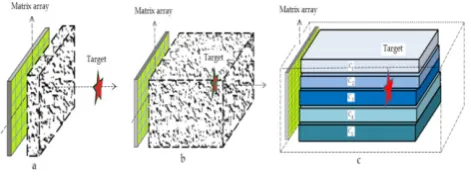
[image:2.595.316.552.224.313.2]propagation medium can lead to significant distortions of the form of images, unwanted artifacts, and very often to the inability of imaging. For long-range sonar the main effects of inhomogeneous medium are associated with refraction of sound waves due to the unknown vertical profile of the sound speed which leads to an ambiguous estimation of target coordinates. For high frequency acoustic imaging systems besides refraction the scattering effects are added. In solids there are various interferential effects caused by generation different types of propagating waves. The simple models of non-uniform mediums which are widely presented in literature are presented on Fig.1.
Figure 1. Different models of non-uniform mediums
The first model (1a) suggests that some inhomogeneous layer is placed between array (for example 2D matrix array in general case) and target; but array and target themselves are placed in uniform medium. Very often such inhomogeneous medium is considered as a phase screen or combination of phase screens with random scatterers of different dimensions which change phases of passing acoustic waves. Possible absorption is usually ignored. Scattering causes deformations of wave fronts and images can be distorted or can disappear at all. More complex model (1b) describes the case when array and object are in a medium filled with random scatterers. The model (1c) describes the typical situation in ocean acoustics – multipath propagation of sound waves where refraction of waves is due to non uniform sound speed profile in a vertical plane. In some cases this model is more complex when it is necessary to take into account the scattering of sound on the sea surface or some effects because of complex bottom structure. Unfortunately, as it is often the case in practical applications of acoustical imaging all of these effects may be present simultaneously.
Another very serious problem is the spatial-time fluctuations of the various parameters of the inhomogeneous medium. The actual sound propagation environments are not "frozen" and can vary due to various factors. These fluctuations are most typical for oceanic underwater acoustics; however, they also occur in other fields of application of acoustical imaging.
that the basic approaches to this problem have been borrowed from optics and radio communications, where the similar problems methods began to develop on 10-15 years earlier. In the mid of 50's astronomers H.N. Babcock (USA,1954) and V.P. Linnik (Russia,1956) has been proposed a method of compensation atmospheric irregularities, later named as "method of phase inversion of the wave front."In optical astronomy this method led to the development of adaptive optics, and in radar and underwater acoustics, where correlation processing of broadband signals was used, the modification of this method was named a "matched signal processing”, “matched filtering” or “matched spatial filtering”.[4,6]. It was based on preliminary calculations or measurements of the transfer functions of the non-uniform propagation channel sound (Green's functions) with subsequent correction of the amplitude and phase coefficients in the elements of receiving and transmitting arrays,[3].
In 1955 Van-Atta- Strahler presented the similar method of phase inversion for underwater acoustics and radio communications where his design is known now as Van-Atta array [7-9]. This array does not require complex signal processing and is a passive multi-element array which provides phase inversion of coming radio (or acoustic) waves automatically using passive elements. Today Van-Atta arrays are widely used in radio communications and mobile. In the end of 80th similar to Van Atta’s method was suggested by M. Fink et al and named “time reversed acoustics”[10,11]. Despite the great similarity of matched filtering and time inversion method, these two methods of image reconstruction differ from each other. Detailed analysis of these two approaches is made by V.A. Zverev [12] where he underlined that matched filtering is a "holographic method”, because it is a spatial processing, and time inversion is based only on the temporal signal processing and it is applicable to both the multi-element array and a separate point transducers.
The physical sense of phase inversion method for quasi-monochromatic signals can be illustrated by the next example. Suppose we see an object through a transparent glass cylinder. Then cylinder is crashed into two halves. The surface of the first halve of the cylinder became irregular and viewed image of the object will be distorted. However, if the second half of the cylinder is preserved, they can be connected and viewed the image of object will be not distorted again. From this simple example not simple conclusions are followed, however, and the most important are the following:
In the real unknown and heterogeneous environment "a form of surface of broken cylinder" or a form of distorted wave front passed through this medium is unknown. Consequently, we need to find a way how to calculate or how to measure this wave front. This is the first problem.
These measurements or calculations must be executed with very high “phase” accuracy – the connection of two halves of cylinder must be very
accurate, otherwise the quality of image will be poor. This is the second problem.
Even if we can accurately calculate or measure transfer functions, one problem is still remains: fluctuations. Real sound propagation channel is not "frozen" and its properties may change over time with some speed, and hence, the shape of the wave front will also vary randomly. Therefore, the speed of measurements and speed of signal processing will depend on speed of fluctuations.
What should be the accuracy of such measurements? Specialists on array systems know well that the spreads of individual phases in the array elements must not exceed the
value of λ/32, (λ/64 is better). The same requirements are
true for primary electronics: spreads of phases in amplifiers must not exceed +/-50 at the highest frequency. The requirement of high precision of phase measurements is complicated by another problem. In order to realize high accuracy we need a very high signal/noise ratio. It is surprising that in spite of these difficulties, the stated problems were first successfully implemented exactly in coherent optics, although the lengths of optical waves by several orders of magnitude smaller than in acoustical imaging and hydroacoustics. Modern adaptive optical telescopes can adjust the form of mosaic mirrors only for 25-35 microseconds; this is the time of "frozen turbulence" in atmosphere, which distorts the image. In long range radio communications and even in modern cell telephony in multipath propagation the similar tuning is performed with very high speed.
However, in underwater acoustics matched signal processing got very limited application. In the long-range sonar, using combined transmitting/receiving arrays these methods can not operate.Because we do not know the position of the target we can not measure its transfer functions in all possible positions, other words we have no information about the position of reference point. Even if this position is known for some private cases, time of propagation of signals can be more than time of variation of parameters of environment. Calculations of transfer functions are possible but for very limited types of waveguides and for real ocean channels can not provide estimation of wave fronts with necessary accuracy.
information for subsequent adjustment of the amplitude and phase parameters of array. The problem of the reference signal was the most important in the adaptive optics and it is directly related to the so-called "phase problem" in optics. It is therefore quite natural that especially in the optics some alternative methods of image restoration, which do not require the use of a physical reference source, have been developed and are developing in the present time. These interesting and new methods will be considered later.
2.1. Matched Filtering in Ocean Acoustics
In order to emphasize the difficulty of matched signal processing in multipath waveguide let’s consider the following example: let’s ocean waveguide has a depth hac
=100m and point source with a frequency f = 3 KHz( λac = 0,5 m) is placed on the distance Lac = 1000 m. Now imagine that we use the optical model of this waveguide on optical
wavelength λop= 0,5μm. Using scaling factor proportional to relation of these wavelengths the optical model of a waveguide will have dimensions: spacing between two mirrors: hop = 100/106 = 10 mm and Lop = 100 mm [13]. Now let’s place light source between these two mirrors and look into their end face. Obviously we will see hundreds images of dots. Why? The answer is very simple: our vision is adapted to imaging in a free space and from a mathematical point of view, our eyes carries out Fourier transformation. But this operator is a not correct inverse operator for waveguide, or other words our signal processing is not matched with a waveguide. Therefore the results are multiple images of source and high ambiguity of positioning of the source. The wavelengths of real underwater sonar arrays are more modest than in optics but such ambiguity will constantly present in a vertical plane.
[image:4.595.326.541.194.276.2]Let’s present some experimental examples. Multichannel record of noise signals received on horizontal array from point noise source is presented of Fig.2. Sound source was on the distance about 35 km from array. The wavelength of array is about 75 on a central frequency, sea state - 4; hydrology is a near surface channel of sound propagation. One can see that the wave fronts of coming waves are plane and in a horizontal plane there are no problems with reconstruction of the image of point noise source: the inverse operator is a Fourier transformation. Therefore in a horizontal plane the medium of sound propagation is uniform.
Figure 2. Multichannel record of wide band noise signals from N
elements of linear array. Number of channels N=120.
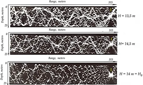
[image:4.595.314.551.446.587.2]A completely different situation arises when the linear receiving array is located in the waveguide vertically, Fig.3. The experiments were conducted on Ladoga Lake with depths of 30-35 meters [14]. The vertical flexible array overlapped almost the waveguide on depth and contained 24 hydrophones with a spacing of 1.25 m. Transducer, generated simple pulse signals and was placed on the depth 14 meters anddistancesR1 = 315 meters and R2 = 930 meters. Wind speed was less than 0.3 m / sec.
Figure 3. Multichannel record of N signals from point source received on a vertical linear array
It is clearly seen from Fig.3 that form of coming wave front is not plane and we can use MSP to reconstruct the image of point source. The detail procedures are described in [14] and we will present only final results. On Fig.4 some results of computer simulation of matched filtering for stated conditions are presented. A possible source depth varied in increments of 0.5 m and best match happened at a depth of 14 m, equal to the true depth, but that is obvious. The calculations took into account all 22 running normal waves.
Figure 4. Simulation of matched filtering at variations of depth of the source. Yellow arrow marks the initial position of point source
[image:4.595.58.296.637.721.2]Figure 5. Experimental results of matched filtering.A. H=13,5 m ( no image,b. H=14 m no image), c. H=15,2 m, image is reconstructed. Red star marks the real position of source. Yellow arrow marks the position of reconstructed image
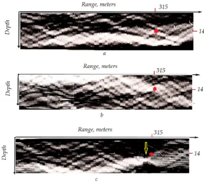
[image:5.595.318.546.221.294.2]These experiments were conducted in sufficiently «hothouse» conditions when previously it was possible to carry out all geometrical measurements. And even in these conditions, we can see that the parameters of the adaptive processing must be carefully selected. Some data on experiments on matched filtering in long range underwater acoustics are presented below [15]. The experiments were conducted in a Mediterranean Sea on frequency F = 30 Hz. The max spacing between transmitter and receiver was 28 km. The depth of transmitter was H = 150 m. Method of aperture synthesis was used to select and measure normal modes. The receiver was a 40 meter vertical cable array with 48 hydrophones. During the drift of the vessel array was continuously went down at a predetermined rate. Controlling the distance between two vessels was performed by standard radio navigation aids and measured coordinates were used for further data correction. Maximum length of the synthesized aperture was L = 500 m. First of all we will demonstrate temporal records of propagating signals for different distances between vessels. The first record, Fig 6a, is made on a short distance R1= 650 m and one can see two wave fronts. The first wave has a spherical front and this is a direct wave from transducer. Because the transducer had very wide directivity on F=30 Hz the second wave is the reflection from the surface. Sloping straight lines are the ship's noise.
Figure 6. Records of measured wave fronts from transducer on different distances between vessels. a. R= 650 m, b.R=15,6 km. c. R = 28 km.
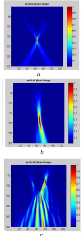
It is clearly seen how multiray propagation is developing on different distances from source of sound. On the next Fig.7 the result of MSP is presented. In spite of that estimated number of running normal modes with a appropriate intensity was about over dozen experiments showed that only 4-5 normal modes could be coherently combined, Fig 7. The rest of the normal waves created additional noise and were uncorrelated. Note that despite the small number of summed modes, images of calculated filed and experimentally reconstructed field are in a good agreement, although the spatial resolution is not high.
Figure 7. Calculated inversed filed (a) and reconstructed image of source (b)after matched filtering for number of normal modes N=5 Green and red dots correspond to the initial coordinates of source,
On the one hand the above results demonstrate the principal possibility of the matched filtering in the ocean waveguides for which the transfer functions can be pre-calculated. But on the other hand, the problems of practical implementation of MSP are obvious. It seems that the practical application of the matched signal processing in underwater acoustics at large distances using the dual-mode of reception is problematic so far. The validity of this statement is confirming by many works of researchers, the overwhelming number of which is devoted to the use of MSP and TRA for spaced receiving/transmitting systems in different environments [50-52].
2.2. Matched Filtering in Medicine Acoustics
Ultrasound is widely used in medicine applications as for therapy and surgery as for diagnostics of internal organs. In the majority of medicine applications the medium of propagation of ultrasound waves is supposed similar to uniform medium and this permit to use more and less standard schemes of ultrasound imaging on the base of 1D or 2D arrays. Unlike underwater acoustic imaging where array dimensions are smaller than the distance to the object in medical applications, they can be comparable. Therefore, at such distances it is necessary to use focused arrays to provide a better resolution. However, this difference is not principal and in ultrasound therapy and surgery, for example, focused arrays are widely used.
[image:5.595.66.291.642.730.2]bone is characterized by very high absorption of sound on high ultrasound frequencies and the low boundary of bone is irregular.
Figure 8. Fragment of skull bone,[29]
The complex structure of the skull leads to strong defocusing of the images of soft tissues, the unpredictability of their position, the emergence of multiple reflections of ultrasonic waves from the surfaces of the bone and very low contrast of images. To all mentioned effects one should add an additional damping of ultrasound in the hairline. Numerous studies of ultrasound transcranial diagnostics [17-22] indicate that the MSP and TRA are possible methods of obtaining images of the brain structures, though there is problem of reference point.
Different researchers proposed some perspective approaches to bypass this problem. K. Hynenen [23,24] suggested preliminary to receive X-ray image of skull bone and then use these data for calculations of irregular form of low bound of skull bone and building of matched filter. The advantage of this method is a very high accuracy of measuring of the form of low boundary of skull bone. From other side the disadvantages are the necessity to use very precise navigation of ultrasound sensor to install it exactly in an appropriate place of skull and additional X-ray inspection of a patient. Other approach based on combination of MRI technique and TRA is discussed in [25,26]. It is necessary to note that combination of TRA with X-ray or MRI inspection is a good approach in ultrasound surgery, for example HIFU method. But combination of different radiation diagnostic procedures with ultrasound inspection is a not appropriate for ultrasound medicine diagnostics, because in that case it is simply not needed.
The perspective possible approach is to use the same ultrasound methods of measuring different parameters of skull bone[27-30]. One can use as multielement array or scanning single transducer. Acoustical methods permit to measure the local thicknesses of skull bone and local acoustical impedances, and in particular local sound speed and attenuation, details of which completely defines the complex transfer functions of bones to build a matched filter. In [28] it has been proposed to use spaced transmitter and receiver to minimize the effects of multiple reflections in the cranial bones. Below we will present some experimental results on transcranial ultrasound imaging [27-29].
Some simulation results of different effects in thick skull bone are presented on Fig.9,[29]
The part of experimental set-up is shown on Fig.10. Left image is a fragment of natural skull bone with average thickness 12 mm. Right image is a container with a
phantom of skull bone (left) and a fragment of skull bone. Transducer had a central frequency 1,7 MHz and 128 elements [28].
Figure 9. Simulation of different effects in a skull bone. a. Uniform medium, bone is absent. b. Two layered bone, refraction effect and defocusing because of non uniform internal boundary. c. Combination of two layered skull bone with intermediate scattering layer and irregular internal boundary
[image:6.595.72.280.122.168.2] [image:6.595.323.540.601.728.2]Next Fig.11 demonstrates the effect of matched filtering. The objects were 5 thin nylon strings with a thickness 0, 8 mm placed in an angle sector 360on different distances from transducer with central frequency F=1,7 MHz
Figure 11. Experimental results of acoustical imaging of point targets through fragment of skull bone. a. Standard imaging in B-mode. b. Image after matched filtering.
All mentioned effects of influence of non uniform skull bone are clearly seen on Fig 11a. Images are strongly defocused, their angle position is wrong and near distances are occupied by multi reflections of sound between skull
bone boundaries. Matched filtering procedure eliminates these effects, though some part of near field reverberation is still seen. Matched filtering procedure in transcranial imaging was tested in vivo [28]. The object of research was
a sinus venarum, a big venous blood vessel passing through
the middle of the skull. This object is interesting because its cross section looks like triangle, Fig.12a and Fig.12b.
It is seen that the ultrasonic image reproduces the "triangular shape” of the vessel and some other internal brain structures are clearly seen. Note that X-ray angiography image reproduces blood flow and ultrasound image reproduces the internal structure of vessel, its walls.
Researches on matched filtering processing in heterogeneous environments and rapidly developing and there is no doubt that they will receive a wide practical application especially in ultrasound medicine diagnostics and non-destructive testing. Nevertheless, these methods have very serious limitations associated with the presence of temporal fluctuations of environmental parameters. The role of these fluctuations is particularly significant in the underwater imaging. TRA can solve this problem only partly, because it does not require the knowledge of transfer functions as in matched filtering procedures,[30]. However, the "payback" for such possibility is the “spacing” of receiving and transmitting points that is impossible in many practical cases.
[image:7.595.67.287.132.315.2] [image:7.595.166.451.418.659.2]3. Methods of Acoustical Speckle
–Holography
Considered methods of acoustical imaging in heterogeneous environments are based on the possibility of separating coherent and most stable part of the signal from the received fields, which in the process of propagation retains its shape and phase relationships. All other "additives" are regarded as interference. In a homogeneous medium such interference is independent noise of environments or equipment. In heterogeneous environments, additional noise (waves) is caused by the original signal. Some of these waves scattered by irregularities, create in the received signal amplitude and random phase modulation, which has a multiplicative character. It is this type of interference, stationary or non-stationary, causing unpredictable deformation of the wave fronts, which can not be suppressed by increasing the intensity of the signal and matched filtering becomes not effective.
Does this mean that in a non-uniform and unknown propagation we can not get information on the subject, for example, to measure its current position, speed, or, finally, to restore its image? In the limits of the classical linear signal processing based on detection of the coherent component, in general, stable solutions are not found, and, possibly, could not be found. However, it appears that much of the information can be obtained by processing and analyzing only the multiplicative random component of the received field, i.e. namely the component which in the classical theory of detection is considered as the most "harmful". However, signal processing techniques are becoming non-linear.
Yu.Lysanov [31] was probably the first who suggested in 1967 the idea of extracting useful information from the acoustic fluctuations. His method of précised estimation of velocity and shifts of sound source was based not on the traditional detection of the coherent echo-signal reflected from the floor, and on the evaluation of the correlation function of fluctuations of the sound field scattered by bottom irregularities. Other words random fluctuations of scattered signals were the source of valuable information. Around the same time, speckle holography or speckle interferometry in coherent optics was developed, which allowed very precise measurement of various parameters of the object [32].The useful information was extracted not from the initial image of the object, and from the noise image of object in which the original image of the object was transformed using a diffuser. Information about parameters of object was extracted from the correlation functions of the scattered fields. This approach seemed paradoxical for many professionals - opticians in that time, because for example, the object was covered with diffusive glass to measure it’s very small shift and the image itself disappeared. However, the accuracy of such measurements was very high. Later the similar ideas of speckle-interferometry were proposed by Layberi in optical astronomy to measure the diameter of the double stars that could not be resolved due to atmospheric
turbulence[33].In ocean acoustics, based on analogies with the dark-field optical method of dark field, V. Zverev developed a method called "reversed aperture synthesis in the dark field" [34,35] in which coherent and stable component of the signal was suppressed, and useful information was extracted from the fluctuating component. Later developing this idea, he proposed a method of beamforming of flexible towed array which shape could randomly vary, but measuring of the shape was not necessary. Another methods of acoustical imaging in heterogeneous and scattering medium, based on the methods of nonlinear phase speckle interferometry has been proposed and developed in [37-43], where it was shown that it is possible to uniquely recover the trajectory of a sound source moving in a ocean waveguide or in strongly scattering medium, and with an accuracy of the diffraction resolution of the array. In [41], this approach was applied for visualization of fluid flow through inhomogeneous layers, and in [42] the ability of acoustical imaging of extended objects, located at the inhomogeneous scattering medium was demonstrated. We emphasize once again that in the methods of speckle interferometry or speckle holography the information about the object and its parameters is extracting from the fluctuation part of the received field. These fluctuations can be caused by natural reasons, but they can be created artificially, for example, by small and accidental movements of the transmitter or receiver. The main advantage of these methods of image reconstruction is that they do not require a detailed description of the parameters of an inhomogeneous medium, in comparison with methods of matched signal processing.
3.1. Principle
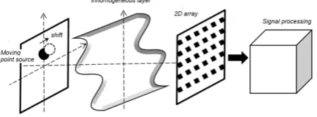
Let’s explain the principle of speckle interferometry on a simple example, Fig.13
Figure 13. Measuring of the trajectory of point moving source through inhomogeneous layer
Let inhomogeneous scattering layer is positioned between the moving point sound source and a 2D receiving array, and we need to measure the trajectory of this source. Properties of the inhomogeneous layer are such that it completely distorts the wave front from the source and the registered fields look like noise images due scattering and so the usual beamforming is senseless. In a moment of time t = t1 let’s
register the intensity of scattered field I1(x ,y) on array. In
[image:8.595.319.544.520.603.2]it’s position and we register the second distribution of intensity I2(x ,y). This second image looks like the first image
and visually differences between the two images are not detectable. It turns out that if the shift of the point source ∆
satisfies to certain conditions, of which we shall speak later, the two intensity distributions are correlated. Well known Young’s fringes are the result of such correlation, Fig.14.
Figure14. Reconstruction of the trajectory of sound source by speckle interferometry method
Having the result of correlation it is simple to reconstruct the image of point source using Fourier transformation of Q. Note that detail information about parameters of scattering layer to reconstruct the image was not required.
3.2. Near Field Underwater Imaging
[image:9.595.77.273.166.346.2]Below some experimental results of underwater acoustical imaging are presented [42].In this work acoustical lens camera with 2D PZT was used on frequency 1 MHz;2D array had 95*95 elements. Perspex screen with random holes of different diameters was placed in front of lens. Point source located at a distance of 7 meters mechanically moved along the rectangular "spiral" trajectory in the transverse plane.
Figure 15. Acoustical lens camera (a), Phase screen with random holes
Some experimental results are presented on Fig 16. Two types of screens were used. One of them had holes with diameters more than a wavelength and the second screen had small holes with diameters about wavelengths.
One can see that for the Screen1 the image of the trajectory reconstructed by standard beamforming, though
being distorted, is slightly recognizable. For Screen 2 standard beamforming can not reproduce the trajectory at all. Speckle processing reconstructs trajectory for both types of screens with a good quality.
Figure 16. Reconstruction of source trajectory. a. Screen 1, standard lens imaging (Fourier beamforming). b. Screen 1.Speckle-interferometry processing. c. Screen 2, standard lens imaging (Fourier beamforming).d. Screen 2, Speckle-interferometry processing
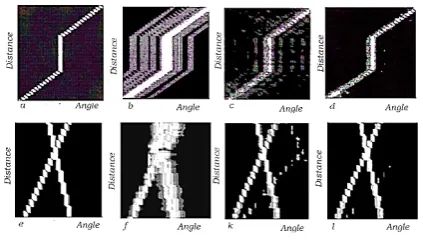
3.3. Far Field Trajectory Imaging in Ocean Waveguides The same ideology of speckle processing can be applied to the detection of the moving point sources in ocean waveguides. It is shown in [39, 40, 43] that in some conditions multi ray structure of acoustic field in a waveguide with vertical stratification of sound speed can be considered as speckle structure and speckle interferometry methods can be used for the detection of moving sound source in ocean channel and measuring its trajectory. It is known that rather long horizontal array can resolve vertical rays especially under big inclination angles. As a result, many responses are formed after array beamforming that causes severe ambiguity in determining the directions of the object. The situation is further complicated when multiple sources are in the surveillance zone of the array. Next Fig. 17 demonstrates the results of computer simulation of possibility of speckle processing to overcome the ambiguity problem not using detail information on sound channel.
[image:9.595.71.286.560.661.2]It is interesting that even in such conditions, speckle interferometry processing allows getting a good image of trajectories of moving ships, though with less contrast and increased noise level. It is clearly seen that after a certain period of time the ships began to move in different courses.
Figure 17. Trajectory of point source moving in ideal ocean waveguide. The length of array is 120 wavelengths. a. Initial trajectory of one moving source. b. Angle spectrum after standard beamforming. c. Result of speckle-processing after 20 iterations. d. Result of speckle processing after 50 iterations. e. Initial trajectory of two moving point sources. f. Angle spectrum after standard beamforming. k. Result of speckle processing after 20 iterations. l. Result of speckle processing after 50 iterations
Figure 18. Detection with a flexible array. a. Standard beamforming. b. Speckle-processing
3.4. Speckle Imaging of Extended Objects through Scattering Medium
The described methods of speckle interferometry imaging referred to the case of reconstruction of acoustic point objects. For such objects the information on intensities of scattered fields is only required. Is it possible, using the same methods, to obtain images of extended objects, located in heterogeneous environments? The results of [] show that a similar ideology can be applied, but under certain additional conditions. The first condition is that the received field must have partial temporal coherence and time of registration of this field must be less than the time of partial coherence. Other words the information on intensities of field is not sufficient and we need some phase information. Moreover if we have this phase information the information on
amplitudes of scattered field is not obligatory. The second condition is that model of object must be described by a set of independent scattering points. Finally, the third condition is that during the time of partial coherence (time of registration) the object and receiver should not change their relative position. If these conditions are met, then the process of imaging of the extended object through inhomogeneous medium is the following []. The scattered field of the object
S(x,y,t)can be presented as the sum of scattered waves
) , , ( )
, ,
(x y t A x y t
S =
∑
∗i (1)Where А*
I (x,y,t)are complex functions, diffracted on the
phase inhomogeneities of the layer Ψ(x,y) and transformed into a random field P(ξ,χ,t), which can be recorded as a convolution
) , ( ) , , ( )
, ,
(ξ χ t =
∑
A* x y t ⊗Ψ x−ξ y−χP i (2),
Let us now assume that at a certain time t1 we separated a
single phase component from the interferential pattern as a whole
Ф1 (ξ,χ) = arg |P1(ξ, χ)|2 (3)
and then in a time period t2= t1 + Δt made a second measurement
Ф2(ξ,χ) = arg |P2(ξ, χ)|2 (4)
During this time Δt the image shifted to a value less than length of coherence lcoh. Now let’s form a diminution
ΔФ(ξ,χ) = Ф1(ξ,χ) – Ф2(ξ,χ) (5)
and reconstruct the image using this differential phase distribution. In this case the term “image reconstruction” means that we use a Fourier transformation of (5). Because the inhomogeneous layer introduces multiplicative noise to the spatial distribution of the signal, the operation (5)
subtracts all the constant phase shifts acquired by the signals
passing the inhomogeneous layer.
As we use the convolution of two fields of the initial object, we will not, of course, reconstruct its actual image. The processed image will consist of separate dots with random distribution and random amplitudes. The number of points will be also random. What is important, however, is that the dots will be located only in the area occupied by the initial object. If we will periodically repeat these calculations (iterations) and average (sum) output images, the pattern will be filled with new dots and smoothen out; the initial image of the object will be the end result of such averaging. Note that the reconstruction of the image from the phase difference does not use information on amplitudes of scattered fields used, although the reconstructed image will contain complete information about all the dynamic range of intensities.
[image:10.595.71.283.146.266.2] [image:10.595.96.259.355.522.2]angiogram of the blood vessels of the brain. Image of two vessels in the white square is aneurysm, which is one of the most dangerous diseases.
Figure 19. X-ray angiography image of aneurism in brain vessels.
Computer simulation results of ultrasound imaging of aneurism through a thick skull bone using nonlinear speckle holography are presented in Figure 20. The thickness of the bone has been 12 mm, and phases of echo-signals scattered on the formed elements of blood (erythrocytes) randomly varied from 0 to 2π. Precisely these signals carry useful
[image:11.595.92.263.367.532.2]information, and all the permanent stable phase shifts caused by the heterogeneity of the bone are suppressed.
Figure 20. Simulated ultrasound speckle images of aneurism through thick bone with a different number of iterations,5, 15, 25 and 50 accordingly
Figure 21. Ultrasound imaging of blood flow on biological phantom. a. Standard Doppler image (courtesy of Medelkom Ltd), b. Speckle image.
Experimental results of blood flow imaging on biological
phantom are presented on Fig.21. Left image is a standard Doppler imaging and the right picture – is a speckle image. Standard Doppler image reproduces blood flow and some static structures while speckle image plays only blood flow, [45]
4. Do We Need Information on Phase?
The diffraction theory states that in order to reconstruct the image of an object located at some distance from the plane of observation, it is necessary to register the complex amplitude-phase distribution of the field scattered by the object. In optics, this can only be done by holographic (interferometry) registration, and in acoustics, complex field can be recorded directly as acoustic transducers are linear. A registration of field with phase accuracy always needs overcoming a number of complex physical and technical problems. For this reason, over the decades, many researchers have tried to answer the question: is it possible to restore the image of the object by recording only the intensity of the scattered field? This problem in optics was named as "phase problem",[46 - 52]. Apparently it is impossible to find more and less stable solutions in the limits of linear theory of diffraction and linear signal processing methods. The appearance of speckle holography, especially with diffuse scatterers, again revived interest to the phase problem. More in-depth studies of the speckle patterns and their unique features have led to propose several methods of imaging, recording only the intensity of the scattered field. Recently, in coherent optics three different methods of image reconstruction through a scattering medium were offered [47-52]. The first method can be called “random selection local phases of speckles”[47, 48], the second method [49]is based on the specific properties of speckles, which enable, by the registered intensity to simulate complex field, like the original, and, finally, the third method does not require registration phase information,[52]. Though these methods have been proposed in optics they are, in author’s opinion, may be of great interest to acoustics, because the problem of registration of phase distributions with high accuracy is no less actual and for acoustical imaging systems due to the big number of channels in 2D matrix arrays, and comparability time of flights of echo-signals with time scales of phase fluctuations in real environments. And secondly as it will be clear later the practical implementation of suggested methods in acoustics is much simpler than in optics due to linearity of transducers and low sound speed.4.1. Random Selection of Local Phases Versus Matched Filtering
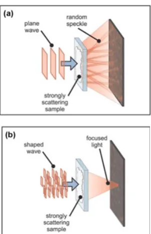
[image:11.595.82.277.573.704.2]scrambling of the field makes it impossible to control wave propagation using the well-established wavefront correction methods of adaptive optics. Authors [47,48] demonstrate focusing of coherent light through disordered scattering media by the construction of wavefronts that invert diffusion of light. Their method relies on interference and is universally applicable to scattering objects regardless of their constitution and scattering strength. Authors [47] envision that, with such active control, random scattering will become beneficial, rather than detrimental, to imaging. The described method is for optical focusing through scattering medium, but it is fully applicable to ultrasound imaging. The central idea of the method is demonstrated on Fig. 25 [47]
Figure 22. Design of the experiment. (a) A planewave is focused on a disordered medium, and a speckle pattern is transmitted. (b) The wavefront of the incident light is shaped so that scattering makes the light focus at a predefined target.[47]
Wavefront correction is performed as follows. The experimental setup for constructing such wavefronts is shown in Fig. 23.Light from He-Ne laser is spatially modulated by a liquid-crystal phase modulator and focused on an opaque, strongly scattering sample S. The number of degrees of freedom of the modulator is reduced by grouping pixels into a variable number Nofsquare segments. A CCD camera monitors the intensity in the target focus and provides feedback for an algorithm that programs the phase modulator.
In Fig. 24 the intensity pattern of the transmitted light is presented. In Fig. 24(a)one can see the pattern that was transmitted when a plane wave was focused onto the sample. The light formed a typical random speckle pattern with a low intensity. Then the wave front is optimized so that the transmitted light focused to a target area with the size of a single speckle. The result for a wave front composed of 3228 individually controlled segments is seen in Fig. 24(b),
where a single bright spot stands out clearly against the diffuse background. The focus was over a factor of 1000 more intense than the non optimized speckle pattern. By adjusting the target function used as feedback it is also possible to optimize multiple foci simultaneously, as is shown in Fig. 24(c)where a pattern of five spots was optimized. Each of the spots has an intensity of approximately 200 times the original diffuse intensity. In Fig. 27(d)we show the phase of the incident wave front corresponding to Fig. 24(c). Neighboring segments are uncorrelated, which indicates that the sample fully scrambles the incident wave front. The optimal phase for a single segment is changing at a time by cycling its phase
from 0 to 2π. For each segment the phase at which the target
intensity is the highest is stored. At that point the contribution of the segment is in phase with the already present diffuse background. After the measurements have been performed for all segments, the phase of the segments is set to their stored values. Now the contributions from all segments interfere constructively and the target intensity is at the global maximum
[image:12.595.331.535.336.438.2]Figure 23. Schematic of the apparatus. A HeNe laser beam is expanded and reflected off liquid crystal spatial light modulator (SLM). Polarization optics select a phase mostly modulation mode. The SLM is imaged onto the entrance pupil of the objective. The shaped wavefront is focused on the strongly scattering sample (S), and a CCD camera images the transmitted intensity pattern.[47]
Figure 24. Transmission through a strongly scattering sample consisting
of TiO2 pigment. (a) Transmission micrograph with an unshaped incident
[image:12.595.325.538.514.661.2]Certainly this procedure of phase selection is a time consuming and authors reports that general time was about 5400 sec using all controlled segments of space modulator. It is clear that the same approach can be applied to high-frequency ultrasound imaging where such feedback can be simply organized by digital processing. In ultrasound case the variations of local phases on elements of transducer can be performed with very high speed and we do not need priory information about parameters of scattering medium.
4.2. Speckle Hologram with a Virtual Reference Wave Another method was published in [49] and was named “optical holography with virtual reference wave”. The authors draw attention to the fact that the phases of neighboring speckles in Fourier holograms registered
through diffusive screen, are abruptly changing on π. This
property of speckles on the assumption that the object is axisymmetric, and its scattering field is characterized by delta correlation, made possible to use virtual reference wave, i.e. modeled. Thus the procedure of recording of hologram and its reconstruction looks as follows: a) Registration of intensity of Fourier hologram of object through diffusive screen and it’s digitizing. This hologram looks like classical speckle pattern, Fig.22b,b) Formation of interference fringes at a predetermined spatial frequency and imposing of these fringes on the speckle pattern, Fig.22c
Figure 25. Fragments of Fourier speckle holograms. a. Fragment of speckle hologram with optical reference wave. b. Fragment of Fourier speckle hologram registered on intensity. c. Fragment of Fourier hologram (b) with superimposed interference fringes. [49]
From Fig.25a one can see that optical speckle hologram consists of random black and white spots (speckles) modulated by interference fringes generated by optical reference wave.
In the transition from speckle to speckle the fringes shifted to a certain part of their period, since the phase in the speckle pattern varies. The contrast of the interference fringes is determined by the ratio of the amplitudes of the object and reference waves in each speckle. Thus, information about the amplitude and phase distribution of the object field is encoded in the spatial position of speckles, their form, position and contrast of interference fringes. The intensity of speckle structure registered on intensity is presented on Fig.25b and this pattern does not contain interference fringes. After imposing of interference fringes on hologram Fig. 25b, the resulted virtual hologram, Fig.25c, is formed which structure is very similar to structure of analogue optical hologram on Fig. 25a.Some examples of image
reconstruction are presented on Fig.26.
Figure 26. Reconstruction of image. a. Initial object. b. Reconstructed image from optical hologram. c. Reconstructed image from virtual hologram, [49]
It should be noted that the proposed in [49] procedure of creation of a virtual hologram in optics is quite laborious, since it requires digital processing of many thousands of speckles. At the same time, the number of the spatial resolution elements in acoustics is less in hundred times, so the proposed method of reconstruction in acoustics can be performed practically in real time.
4.3. The Iterative Method of Open Resonators
The next method of imaging through scattering medium based on the registration of intensity distribution only was proposed in [52].The approach of the authors [52] is so original and innovative that we will focus on this work in more detail, especially as the quality of reconstruction images is very high. The statement of the problem is the same: image of the object located in a far field zone is observed through scattering medium and intensity of scattered field is registered. It is required to reconstruct the original image of the object using this distribution. Let’s assume that that the object is centered in a plane has a finite size, and its field distribution on the surface is described by scalar complex function f (ρ). Then the field F (ρ1) in the
detection plane of registration of speckle pattern for small angles is related to f (ρ) by integral Fourier relation:
{
i[
x x y y]
}
dxdyy x f A y x
F( 1, 1)=
∫∫
( , )exp ( − 1) +( − 1)And intensity distribution is equal to
) , ( ) , ( ) , ( ) ,
( 1 1 * 1 1
2 1 1 1
1 y F x y F x y F x y
x
I = =
Object field in terms of its phase characteristics is a random statistical field and
> < ≈ + ε ρ ε ρ ρ ρ ρ , 0 ,1 ) ( ) ( 0 f 0
f
[image:13.595.322.538.96.179.2] [image:13.595.71.282.408.486.2]relation between the average intensity and its correlation function 2 1 2 1 1
1 ) ( ) ( )
(r ρ I r I Kρ
I + = + .Using the theorem of
VanCittert – Zernike
− +
=
∫∫
xx yy dxdy L k j y x f A y xK( , ) ( , ) exp ( 1 1)
2 1
1
and further using the obvious relation
+
=
∫∫
xx yy dxdyL k j y x K y x
B( , ) ( , ) exp ( 1 1)
2 1 1
we can receive
[
( 2 ),( 2 )]
ˆ( 2, 2) 2 2 ˆ) ,
(x y I x x y y I x y dxdy
B =
∫∫
− −Where I(x, y) = | f (x, y)|- intensity of object field. Given the fact that object has a finite size, it is possible to find the rectangle directed in some way in the object plane in which function B(x, y) is concentrated relating to its sides. By dividing this rectangle into four equal parts by perpendiculars drawn from the midpoints of adjacent sides, after selecting one of them, we will get a new rectangle, where our object can be located. The boundary points of the object touch all four sides of highlighted rectangle.
It is this rectangle further will be featured as a first mirror of resonator. The second mirror is a region of finite size in the recording plane of speckle pattern. Now the search of steady-state field will hold the following algorithm. Let us choose, for example, as zero approximation the uniform field distribution in the object plane and obtain its Fourier pattern in the plane of speckle pattern. Then, leaving the phase unchanged let’s take a distribution │K (xj,yj)│as
amplitude. Again perform an inverse Fourier transformation. In the object plane the field falling within the above rectangle we will not vary, and all other fields which are not included in the rectangle will be nullified. These iteration procedures are repeating more and more until we will get the reconstructed image. It seems the desired intensity distribution in the object plane (image) is the most appropriate for the generation virtual resonator and in this respect it is its mode: it fits perfectly the rectangular plane, its intensity distribution in the observation plane coincides with | K (x1, y1 | 2, and in the process of iterations it goes into itself. Other possible images with the same distribution| K (x1, y1 | 2 are shifted with respect to the center of the rectangular and shadowed by its edges; so these images will not “survive” during iteration process and can be considered as modes with high losses. More detail description of this procedure one can find in [52].On Fig.27 some reconstructed images are presented following suggested algorithm.
It is interesting to note that in this modeling case the
[image:14.595.326.539.77.144.2]scattering medium has correlation function close to δ- function, so the initial image completely disappeared. Nevertheless the number of iterations was not so big to get reconstructed image of a good quality and we did not use any phase information at all.
Figure 27. Reconstruction of the image of model of aircraft through scattering medium. a. Initial image. b. Registered intensity of image through scattering medium (speckle image). c. Reconstructed image after 35 iterations , [52]
5. Conclusion
The successful solution of the problem of acoustical imaging in heterogeneous environments is very important for a variety of practical applications of acoustic technologies such as underwater imaging, ultrasound medicine diagnostics and ultrasound NDT. As can be seen from the review studies of this problem are developed in two directions. The first direction is methods of wave front inversion in the framework of linear signal processing theory. These methods have a good theoretical basis and potentially can reconstruct the image of the object with the highest authenticity. However, these methods are characterized by a number of restrictions in dual-mode imaging scheme when receiver and transmitter are located in the same place. The necessity to have a “reference point” is a major problem. Despite the impressive experimental results in underwater acoustics, obtained by TRA and MSP, [53- 56] they are still a particular case, when the receiving and transmitting arrays were strictly fixed and sound channel was stable. In fairness, we should note that in underwater communication methods of MSP has been implemented in many commercial systems much earlier, and they give about the same results.
Therefore, methods of MSP and TRA can be widely used in transmission imaging mode or with a combination with other imaging technologies like MRI or X-Ray in ultrasound medicine therapy, for example.
In recent decades, alternative imaging methods based on speckle holography, and speckle interferometry began to develop. Their main advantage is that they can be used in any mode of imaging and require minimum information about the parameters of the propagation channel. Although these methods are often "heuristic" they demonstrate the feasibility of imaging through inhomogeneous medium with sufficiently high quality. Methods, based on the diffuse scattering which is artificially introduced into the processing scheme or natural scattering, induced by medium properties are of a particular interest. According to the results of the cited papers speckle patterns have interesting and unusual features that allow reconstructing images of objects only by registered intensity. Due to scattering the original image is transforming into the noise image, and its specific statistical properties allow restoration the original image.
sound or light) in many cases are not an interfering factor, but, on the contrary, the basis of an entirely new imaging approaches. In particular, it is the effects of scattering of light allowed to put forward and justify the hypothesis of the new mechanism of the primary visual perception which resolves many of the contradictions in the existing theory of vision [62-64]
The unusual properties of the "noisy" speckle holograms are closely related to the more general problem of the influence and the role of noise in imaging, which is also widely discussed in the literature as well-known phenomenon of stochastic resonance when some "noise pollution" of the image significantly increases its contrast [59-61] and that completely contradicts the linear theory of signal processing. The effects of stochastic resonance have been discovered in climate researches, seismology, optics and biology.
Certainly all effects and features of diffusive speckle holograms can be implemented by non-linear signal processing schemes making difficult their mathematical analysis. However, the fact that for a number of models of the scattering medium we can restore the image of the objects of quite complex shapes using minimal phase information and even only the intensity of the registered field indicates the promising of these methods for acoustical imaging in heterogeneous environments.
Acknowledgements
Author is very grateful to the participants of the Prof. S.A. Rybak’s seminar “Acoustics of inhomogeneous media” for fruitful discussions and constructive suggestions.
REFERENCES
[1] Baggeroer, A. B., Kuperman, W. A., and Mikhalevsky, P. N. (1993). An overview of matched field methods in ocean acoustics. IEEE J. Oceanic Engng., 18:401–424
[2] N.V. Zuikova, V.D. SvetMatched filedprocessing in waveguides with sound velocity profile. Akusticheskij Zhurnal ( Review) ,1993, 39, issue 3 p.389-403
[3] Baggeroer, A. B., Kuperman, W. A., and Schmidt, H. (1988). Matched field processing: Source localization in correlated noise as an optimum parameter estimation problem. J. Acoust. Soc. Am., 83:571–587.
[4] Krolik, J. L. (1992). Matched-field minimum variance beamforming in a random ocean channel. J. Acoust.Soc. Am., 92:1408–1419.
[5] Arthur B. Baggeroer, William A. KupermanMatched Field Processing in Ocean Acoustics Acoustic Signal Processing for Ocean Exploration, NATO ASI Series Volume 388, 1993, pp. 79-114
[6] W.A. Kuperman and H.C. Song,Integrating Ocean Acoustics
and Signal Processing, Advances in Ocean Acoustics, AIP Conf. Proc.1495, 60-82, (2012); doi:10.1063/1.476590 [7] L.C. Van Atta, Underwater sound reflector. U.S. PatentNo
2,839,735, June 1958, Filled June 8, 1955
[8] L. C. van Atta, "Electromagnetic reflector," U.S. Patent No. 2,908,002, Serial No. 514,040; issued October 6, 1959; filed June 8, 1955.
[9] K. Walther. Model Experiments with Acoustic van Atta Reflectors, JASA, V.34, N.5, 1962
[10] Fink M. Time reversal of Ultrasonic Fields- Part 1: Basic Principles, IEEE Transactions on ultrasonic, ferroelectrics, and frequency control, V.39, N5 1992, p.555-566
[11] Fink, M. (March, 1997). Time reversal acoustics. Physics Today, 50:34–40
[12] V. A. ZverevThe principle of Acoustical Time Reversal and Holography, Acoustical Physics, 2004, V.50, N6, p.792-801 [13] Svet V.D,Zuikova N.V . Optical-digital method of point
source field reconstruction in a layered in homogeneous waveguide,AkusticheskijZhurnal, 33, 3, (1987) p. 493-497 [14] Svet V.D , An experimental reconstruction of a point source
sound field in a waveguideAkusticheskijZhurnal, 36, 4, p. 733-739 (1990)
[15] Dementiev D.A., Svet V.D., Fedotov D.A. Measurement of normal mode parameters by means of aperture synthesis in an oceanic waveguide» AkusticheskijZhurnal, 37, 3, p. 463-468 (1991)
[16] A. Molotilov, Svet V., Baykov S. Ultrasound imaging of cerebrum vessels through thick bones of skull, World Congress on Cerebral Embolism. 1998, November 12-15, New Orleans, LA, USA
[17] Thomas, J.-L. and Fink, M. A. (1996). Ultrasonic beam focusin through tissue inhomogeneities with a time reversal mirror: Application to trans skull therapy. IEEE Trans. Ultrason. Ferroelectr. Freq. Control
[18] J. F. Aubry, M. Tanter, J. Gerber, J. L. Thomas, and M. Fink, Optimal focusing by spatio-temporal inverse. ii. experiments. application to focusing through absorbing and reverberating media." J. Acoust. Soc. Am. 110, 48 (2001).
[19] Marquet, M. Pernot, J.-F. Aubry, G. Montaldo, L. Marsac,M. Tanter, and M. Fink, Non-invasive transcranial ultrasound therapy based on a 3d ct scan: protocol validation and in vitro results." Phys. Med. Biol. 54, 2597 (2009).
[20] Gateau, L. Marsac, M. Pernot, J.-F. Aubry, M. Tanter, and M. Fink, Transcranial ultrasonic therapy based on time reversal of acoustically induced cavitation bubble signature." IEEETrans. Biomed. Eng. 57, 134 (2010).
[21] F. Aubry, L. Marsac, M. Pernot, B. Robert, A.-L. Boch,D. Chauvet, N. Salameh, L. Souris, L. Darasse, J. Bittoun,Y. Martin, C. Cohen-Bacrie, J. Souquet, M. Fink, and M. Tanter, High intensity focused ultrasound for transcranial therapy of brain lesions and disorders." IRBM 31, 87 (2010)
[22] Sadler J, Shapoori K, Malyarenko E, Severin F, Maev R.G. Locating an acoustic point source scattered by a skull phantom via time reversal matched filtering. J AcoustSoc Am. 2010 Oct;128(4):1812-22.
amplitude corrections in ultrasound therapy European Patent EP1381430 Kind Code: B1
[24] K. Hynenen. A non-invasive method for focusing ultrasound through the human skull /4/21Physics in medicine and biology, 2002 V.47, 8, pp.1219
[25] K. HynynenMRI-guided focused ultrasound treatments Ultrasonics 50 (2010), 221–229
[26] R. Jones, M. O'Reilly, K. Hynynen Simulations of transcranial passive acoustic mapping with hemispherical sparse arrays using computed tomography-based aberration corrections. POMA Volume 19, (June 2013);
[27] Svet V.D.,Molotilov, A.M,Baikov S.V. «Physical and Technological Aspects of Ultrasonic Imaging of Brain Structures through Thick Skull Bones. Theoretical and Model Studies» AkusticheskijZhurnal, 49, 3, p. 332-341 (2003)
[28] Svet V.D.,Selyanin A.I., Riman V.V., Neiman S.I.,Molotilov A.M.,Baykov S.V., Physical, Technical Aspects of Ultrasonic Brain Imaging Through Thick Skull Bones. 2. Experimental Studies» AkusticheskijZhurnal, 49, 4, p. 465-473 (2003)
[29] R. Maev, V. Svet Ultrasound imaging of brain structures and blood vessels through thick skull bones, Tessonics Corp.,ONR S&T 6.1 Program Review: Stress Physiology July 2007
[30] Sadler J, Shapoori K, Malyarenko E, Severin F, Maev RG. Locating an acoustic point source scattered by a skull phantom via time reversal matched filteringJASA. 2010 Oct;128(4):1812-22.
[31] LisanovYu.P. On temporal fluctuations of sound signals scattered from the sea bottom»AkusticheskijZhurnal, V.13,N 3, p. 401-405 (1967)
[32] Speckle book R. Jones, C. Wykes,Holographicand speckle interferometry,Cambridge University Press, 1989, pp.256 [33] A. Labeyrie Attainment of diffracted limited resolution in
large telescopes by Fourier analyzing speckle patterns in star images.Astron&Astrophys.6,p.85-87.1970
[34] M. J. Cullum Adaptive opticsEuropean Southern Observatory, 1996 – pp. 542
[35] Zverev V.A. Acoustic Dark Field AkusticheskijZhurnal, 46, 1, p. 75-83 (2000) 46, p. 75-83
[36] Zverev V.A., Korotin P.I., Matveev A.L., Satin B.M., Turchin V.I. Inverse Aperture Synthesis in an Acoustic Dark Field,AkusticheskijZhurnal, 46, 5, p. 650-657 (2000) [37] Zverev V.A., Pavlenko A.A.Beamforming for a Flexible
Acoustic Array» 47, AkusticheskijZhurnal, 47, 3, p. 352-358 (2001)
[38] Zuikova N.V., Kondrat'eva T.V., Svet V.D. Application of speckle interferometry to problems of ocean acoustics , AkusticheskijZhurnal, 42, 2, p. 225-231 (1996)
[39] Zuikova N.V., Kondrat'eva T.V., Svet V.D. Ranging an Object Buried under a Layer of ScatterersAkusticheskijZhurnal, 43, 2, p. 187-193 (1997) [40] Svet V.D. Kondratieva T.V. Trajectory estimation of moving
target in the medium with a strong scattering/ Acoustical
Imaging, 1997, V.23, 555-562, Plenum Press. NY.
[41] Zuikova N.V., Kondrat'eva T.V., Svet V.D. Estimating the Angular Movement of a Sound Source in a Multimode Waveguide Akusticheskij Zhurnal, 44, 2, p. 220-225 (1998) [42] Zuikova N.V., Kondrat'eva T.V., Svet V.D. Visualization of Blood Flow by the Method of Ultrasound Speckle Interferometry Akusticheskij Zhurnal, 47, 5, p. 664-670 (2001)
[43] Zuikova N.V., Kondrat'eva T.V., Svet V.D. Acoustic Images of Objects Moving under an Inhomogeneous LayerAkusticheskijZhurnal, 49, 2, p. 183-193 (2003)
[44] Zuikova N.V., Svet V.D., ShatskovYu.A.Determination of the Path of a Sound Source Moving in an Inhomogeneous MediumAkusticheskijZhurnal, 52, 5, p. 655-664 (2006) [45] V.D.Svet1,,T.V.Kondratieva , N.V. Zuikova, S.V. Baykov.
Ultrasound Flow Imaging through Thick Skull Bones in Spaced “Transmitter & Receiver” Mode.Advances in Signal Processing 2(1): 8-17, 2014DOI: 10.13189/asp.2014.020102 [46] Shieh H.M., Byrne C.L. Image reconstruction from limited
Fourier data // J. Opt. Soc. Amer. A. 2006. Vol. 23. P. 2732–2736.
[47] .M. Vellekoop and A. P. Mosk Focusing coherent light through opaque strongly scattering media August 15, Optic letters 2007 / Vol. 32, No. 16
[48] I.M. Vellekoop, A.P. MoskPhase control algorithms for focusing light through turbid media.Optics Communications 281 (2008) 3071–3080
[49] V.P. Ryabukho, B.B. Gorbatenko, L.A Digital Optical Holography with Virtual Reference Wave, Proceedings of Saratov University, 2008, v.8, Physics, N2, Russia
[50] Kolenovic E. Correlation between intensity and phase in monochromatic light // J. Opt. Soc. Amer. A. 2005. Vol. 22. P. 899–906
[51] Bastiaans M.J., Wolf K.B. Phase reconstruction from intensity measurements in linear systems // J. Opt. Soc. Amer.2003. Vol.20. P.1046–1049.
[52] Beldygin I.M.,Zubarev I.G., MikhailovS.I.,.Restoring image of the object on the speckle pattern of its field. Quantum
Electronics. 2001. v. 31, № 6. p. 539-542.
[53] Karim G. Sabra1, Philippe Roux1, Hee-Chun Song1, William S. Hodgkiss1, W. A. Kuperman, Tuncay Akal, and J. Mark Stevenson Experimental demonstration of iterative time-reversed reverberation focusing in a rough waveguide. Application to target detection J. Acoust. Soc. Am. Volume 120, Issue 3, pp. 1305-1314 (2006)
[54] J.-P. Montagner, C. Larmat, Y. Capdeville, M. Fink, H. Phung, B. Romanowicz, E. Cl´ev´ed´e1 and H. Kawakatsu Time-reversal method and cross-correlation techniques by normal mode theory: a three-point problemGeophys. J. Int. (2012) 191, 637–652
[55] Takuya Shimura, Hiroshi Ochi, and Yoshitaka Watanabe Recent experiment results of long-range time-reversal communication in deep ocean J. Acoust. Soc. Am. Volume 131, Issue 4, pp. 3277-3277 (2012);
(2011)
[57] R. Benzi, G. Parisi, A. Sutera, and A. Vulpiani. Stochastic resonance in climatic changes. Tellus,34:10–16, 1982 [58] B. McNamara and K. Wiesenfeld. Theory of stochastic
resonance. Physical Review A, 39:4854–4869, 1989.
[59] K. Loerincz, Z. Gingl, and L. B. Kiss, ‘‘A stochastic resonator is able to greatly improve signal-to-noise ratio,’’ Phys. Lett. A 224, 63–67 ~1996
[60] E. Simonoto, M. Riani, C. Seife, M. Roberts, J. Twitty, and F. Moss,‘‘Visual perception of stochastic resonance,’’ Phys. Rev. Lett. 78, 1186–1189 ~1997
[61] S. M. Bezrukov and I. Vodyanoy, ‘‘Stochastic resonance in nondynamical systems without response thresholds,’’ Nature 385, 319–321 1997
[62] V.D. Svet, About Holographic (Interferometric) Approach to the Primary Visual Perception, Open Journal of Biophysics, 2013, 3, 165-177
[63] V.D. Svet and A.M. Khazen ,Coherent effects in Primary Visual Perception, NOVA Science Publishers, N.Y.USA, 2011, pp.78, ISBN: 978-1-61668-143-2